Download
1 / 27
300 likes | 698 Views
Chapter 13 Return, Risk, and the Security Market Line. 13.1 Expected Returns and Variances 13.2 Portfolios 13.3 Announcements, Surprises, and Expected Returns 13.4 Risk: Systematic and Unsystematic 13.5 Diversification and Portfolio Risk 13.6 Systematic Risk and Beta

E N D
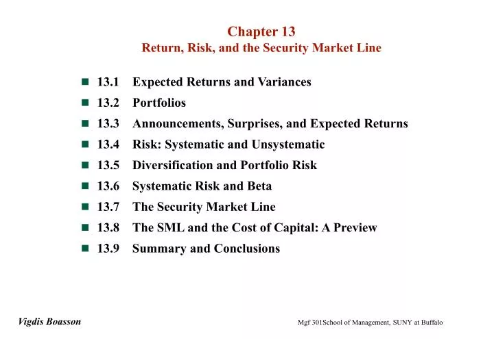
Chapter 13Return, Risk, and the Security Market Line • 13.1 Expected Returns and Variances • 13.2 Portfolios • 13.3 Announcements, Surprises, and Expected Returns • 13.4 Risk: Systematic and Unsystematic • 13.5 Diversification and Portfolio Risk • 13.6 Systematic Risk and Beta • 13.7 The Security Market Line • 13.8 The SML and the Cost of Capital: A Preview • 13.9 Summary and Conclusions Vigdis Boasson Mgf 301School of Management, SUNY at Buffalo
13.2 Expected Returns and Variances: Basic Ideas • The quantification of risk and return is a crucial aspect of modern finance. • And, rational investors like returns and dislike risk. • Consider the following proxies for return and risk: Expected return - weighted average of the distribution of possible returns in the future. Variance of returns - a measure of the dispersion of the distribution of possible returns in the future. How do we calculate these measures?
13.3 Example: Calculating the Expected Return s E(R) = (pi x ri) i =1 pi ri Probability Return inState of Economy of state i state i +1% change in GNP .25 -5% +2% change in GNP .50 15% +3% change in GNP .25 35%
13.3 Example: Calculating the Expected Return (concluded) i (pi x ri) i = 1 -1.25% i = 2 7.50% i = 3 8.75% Expected return = (-1.25 + 7.50 + 8.75) = 15%
13.4 Calculation of Expected Return (Table 13.3) Stock L Stock U (3) (5) (2) Rate of Rate of (1) Probability Return (4) Return (6) State of of State of if State Product if State ProductEconomy Economy Occurs (2) x (3) Occurs (2) x (5) Recession .80 -.20-.16.30.24 Boom .20 .70.14.10 .02 E(RL) = -2% E(RU) = 26%
13.5 Example: Calculating the Variance s Var(R)2 = [pi x (ri - r )2] i =1 pi ri Probability Return inState of Economy of state i state i +1% change in GNP .25 -5% +2% change in GNP .50 15% +3% change in GNP .25 35% E(R) = r = 15% = .15
13.5 Calculating the Variance (concluded) i (ri - r)2 pi x (ri - r)2 i=1 .04 .01 i=2 0 0 i=3 .04 .01 Var(R) = .02 What is the standard deviation?
13.6 Example: Expected Returns and Variances State of the Probability Return on Return oneconomy of state asset A asset B Boom 0.40 30% -5% Bust 0.60 -10% 25% 1.00 • A. Expected returns E(RA) = 0.40 x (.30) + 0.60 x (-.10) = .06 = 6% E(RB) = 0.40 x (-.05) + 0.60 x (.25) = .13 = 13%
13.6 Example: Expected Returns and Variances (concluded) • B. Variances Var(RA) = 0.40 x (.30 - .06)2 + 0.60 x (-.10 - .06)2 = .0384 Var(RB) = 0.40 x (-.05 - .13)2 + 0.60 x (.25 - .13)2 = .0216 • C. Standard deviations SD(RA) = = .196 = 19.6% SD(RB) = = .147 = 14.7%
13.7 Example: Portfolio Expected Returns and Variances • Portfolio weights: put 50% in Asset A and 50% in Asset B: State of the Probability Return Return Return oneconomy of state on A on B portfolio Boom 0.40 30% -5% 12.5% Bust 0.60 -10% 25% 7.5% 1.00 Return on portfolio under Boom = .30 x .5 + (-.05)x .5 = 12.5% Return on portfolio under Bust = (-.10) x .5 + .25x .5 = 7.5%
13.7 Example: Portfolio Expected Returns and Variances (continued) • A. E(RP) = 0.40 x (.125) + 0.60 x (.075) = .095 = 9.5% • B. Var(RP) = 0.40 x (.125 - .095)2 + 0.60 x (.075 - .095)2 = .0006 • C. SD(RP) = = .0245 = 2.45% • Note: E(RP) = .50 x E(RA) + .50 x E(RB) = 9.5% • BUT: Var (RP) .50 x Var(RA) + .50 x Var(RB)
13.7 Example: Portfolio Expected Returns and Variances (concluded) • New portfolio weights: put 3/7 in A and 4/7 in B: State of the Probability Return Return Return oneconomy of state on A on B portfolio Boom 0.40 30% -5% 10% Bust 0.60 -10% 25% 10% 1.00 • A. E(RP) = 10% • B. SD(RP) = 0%
13.8 The Effect of Diversification on Portfolio Variance Portfolio returns:50% A and 50% B Stock B returns Stock A returns 0.05 0.04 0.03 0.02 0.01 0 -0.01 -0.02 -0.03 0.05 0.04 0.03 0.02 0.01 0 -0.01 -0.02 -0.03 -0.04 -0.05 0.04 0.03 0.02 0.01 0 -0.01 -0.02 -0.03
13.9 Announcements, Surprises, and Expected Returns • Key issues: • What are the components of the total return? • What are the different types of risk? • Expected and Unexpected Returns Total return = Expected return + Unexpected return R = E(R) + U • Announcements and News Announcement = Expected part + Surprise
13.10 Risk: Systematic and Unsystematic • Systematic and Unsystematic Risk • Types of surprises 1. Systematic or “market” risks 2. Unsystematic/unique/asset-specific risks • Systematic and unsystematic components of return Total return = Expected return + Unexpected return R = E(R) + U = E(R) + systematic portion + unsystematic portion
13.12 Standard Deviations of Annual Portfolio Returns (Table 13.7) ( 3) (2) Ratio of Portfolio (1) Average Standard Standard Deviation to Number of Stocks Deviation of Annual Standard Deviation in Portfolio Portfolio Returns of a Single Stock 1 49.24% 1.00 10 23.93 0.49 50 20.20 0.41 100 19.69 0.40 300 19.34 0.39 500 19.27 0.39 1,000 19.21 0.39
13.13 Portfolio Diversification (Figure 13.1) Average annualstandard deviation (%) 49.2 Diversifiable risk 23.9 19.2 Nondiversifiablerisk Number of stocksin portfolio 1 10 20 30 40 1000
13.14 Measuring systematic rsisk: Beta Coefficients for Selected Companies (Table 13.8) Beta Company Coefficient (i) Exxon 0.65 AT&T 0.90 IBM 0.95 Wal-Mart 1.10 General Motors 1.15 Microsoft 1.30 Harley-Davidson 1.65 America Online 2.40
13.15 Example: Portfolio Beta Calculations Amount PortfolioStock Invested Weights Beta (1) (2) (3) (4) (3) x (4) Haskell Mfg. $ 6,000 50% 0.90 0.450 Cleaver, Inc. 4,000 33% 1.10 0.367 Rutherford Co. 2,000 17% 1.30 0.217 Portfolio $12,000 100% 1.034
13.16 Example: Portfolio Expected Returns and Betas • Assume you wish to hold a portfolio consisting of asset A and a riskless asset. Given the following information, calculate portfolio expected returns and portfolio betas, letting the proportion of funds invested in asset A range from 0 to 125%. Asset A has a beta () of 1.2 and an expected return of 18%. The risk-free rate is 7%. Asset A weights: 0%, 25%, 50%, 75%, 100%, and 125%.
13.16 Example: Portfolio Expected Returns and Betas (concluded) Proportion Proportion Portfolio Invested in Invested in Expected Portfolio Asset A (%) Risk-free Asset (%) Return (%) Beta 0 100 7.00 0.00 25 75 9.75 0.30 50 50 12.50 0.60 75 25 15.25 0.90 100 0 18.00 1.20 125 -25 20.75 1.50
13.17 Return, Risk, and Equilibrium • Key issues: • What is the relationship between risk and return? • What does security market equilibrium look like? The fundamental conclusion is that the ratio of the risk premium to beta is the same for every asset. In other words, the reward-to-risk ratio is constant and equal to: E(Ri ) - Rf Reward/risk ratio = i
13.17 Return, Risk, and Equilibrium (concluded) • Asset A has an expected return of 12% and a beta of 1.40. Asset B has an expected return of 8% and a beta of 0.80. Are these assets valued correctly relative to each other if the risk-free rate is 5%? a. For A, (.12 - .05)/1.40 = ________ b. For B, (.08 - .05)/0.80 = ________ • What would the risk-free rate have to be for these assets to be correctly valued? (.12 - Rf)/1.40 = (.08 - Rf)/0.80 Rf = 2.67%
13.18 The Capital Asset Pricing Model • The Capital Asset Pricing Model (CAPM) - an equilibrium model of the relationship between risk and return. What determines an asset’s expected return? • The risk-free rate - the pure time value of money • The market risk premium - the reward for bearing systematic risk • The beta coefficient - a measure of the amount of systematic risk present in a particular asset The CAPM: E(Ri ) = Rf+ [E(RM ) - Rf ] x i
13.19 The Security Market Line (SML) (Figure 13.4) Asset expectedreturn (E (Ri)) = E (RM) – Rf E (RM) Rf Assetbeta (i) M= 1.0
13.20 Summary of Risk and Return (Table 13.9) I. Total risk - the variance (or the standard deviation) of an asset’s return. II. Total return - the expected return + the unexpected return. III. Systematic and unsystematic risks Systematic risks are unanticipated events that affect almost all assets to some degree. Unsystematic risks are unanticipated events that affect single assets or small groups of assets. IV. The effect of diversification - the elimination of unsystematic risk via the combination of assets into a portfolio. V. The systematic risk principle and beta - the reward for bearing risk depends only on its level of systematic risk. VI. The reward-to-risk ratio - the ratio of an asset’s risk premium to its beta. VII. The capital asset pricing model : E(Ri) = Rf + [E(RM) - Rf] i.
13.21 Examples Assume: the historic market risk premium has been about 8.5%. The risk-free rate is currently 5%. GTX Corp. has a beta of .85. What return should you expect from an investment in GTX? E(Ri ) = Rf+ [E(RM ) - Rf ] x i E(RGTX) = 5% + 8.5% x .85 = 12.225%