Download
1 / 40
400 likes | 556 Views
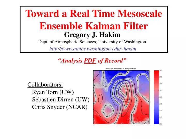
Toward a Real Time Mesoscale Ensemble Kalman Filter. http://www.atmos.washington.edu/~hakim. “Analysis PDF of Record”. Gregory J. Hakim Dept. of Atmospheric Sciences, University of Washington. Collaborators: Ryan Torn (UW) Sebastien Dirren (UW) Chris Snyder (NCAR).

E N D
Toward a Real Time Mesoscale Ensemble Kalman Filter http://www.atmos.washington.edu/~hakim “Analysis PDF of Record” Gregory J. Hakim Dept. of Atmospheric Sciences, University of Washington Collaborators: Ryan Torn (UW) Sebastien Dirren (UW) Chris Snyder (NCAR)
Two Distinct AOR Priorities • NDFD forecast verification. • Nationwide analyses; no critical delivery time? • An a posteriori approach could use max data. • Better centralized for uniformity? • No distribution costs; no hard deadlines. 2) Real-time mesoscale analyses & forecasts. • Regional analyses & short (<12 h) forecasts. • Delivery time critical; use available data. • A distributed/regional approach is helpful? • DA community resource (cf. MM5, WRF, etc.) • EnKF appears well suited.
Summary of Ensemble Kalman Filter (EnKF) Algorithm • Ensemble forecast provides background estimate & statistics (Pb) for new analyses. • Ensemble analysis with new observations. (3) Ensemble forecast to arbitrary future time.
Strengths & Weakness of EnKF • Probabilistic analyses & probabilistic forecasts. • prob. forecasts widely embraced. • prob. analyses don’t yet exist. • account for ensemble variance in NDFD verification? • Straightforward implementation; ~parallelization. • Do not need • background error covariance models. • adjoint models (cf. 4DVAR). • Weakness: Rank deficient covariance matrices. • ensemble may need to be very large. • Many ways to boost rank for small ensembles O(100).
Synoptic Scale Example • Weather Research and Forecasting Model (WRF). • 100 km grid spacing; 28 vertical levels. • Assimilate 250 surface pressure obs ONLY. • Perfect model assumption. • Observations = truth run + noise.
L Cov(Z500, Plow) & Cov (V500, Plow)
Mesoscale Examples • 12 km grid spacing, 38 vertical levels. • 3-class microphysics. • TKE boundary layer scheme. • 60 ensemble members. • Assimilate surface pressure observations. • Hourly observations. • Drawn from truth run plus noise. • Realistic surface station distribution.
Mesoscale Covariances 12 Z January 24, 2004 Camano Island Radar |V950|-qr covariance
Surface Pressure Covariance Land Ocean
Toward a Real-Time Mesoscale EnKF Prototype • Surface observations • (U,V,T,RH, green) • Radiosondes • (U,V,T,RH) • Scatterometer winds • (U,V over ocean, red) • ACARS • (U,V,T)
Summary Ensemble Kalman filter AOR opportunities: • Ensemble mesoscale analyses & short-term forecasts. • Lowers barriers-to-entry for DA. • Regional DA (prototype in progress at UW). • Community DA resource (cf. MM5, WRF). Background Error Covariances: • Automatic & flow dependent with EnKF. • Cloud field analyses no more difficult than, e.g., 500 hPa height. • Optimal ensemble size? • Vary strongly in space & time. • Difficult to assume mesoscale covariances, unlike synoptic scale.
EnKF Sampling Issues • Problem #1: “under-dispersive” ensembles. • overweight background relative to observations. • Solution: Inflate K by a scalar constant. • Problem #2: spurious far-field covariances. • affect analysis far from observation. • Solution: Localize K with a window function.
Analysis-update Equation analysis = prior + weighted observations
Traditional Kalman Filter Problem A forecast of Pb is needed for next analysis. • Problem: Pb is huge (N x N) and cannot be evolved directly. • Solution: estimate Pb from an ensemble forecast. • “Ensemble” KF (EnKF).
Current DA and Ensemble Forecasting 3D/4Dvar:Pbis~ flow independent. • Assumed spatial influence of observations. • Assumed field relationships (e.g. wind—pressure balance). • Pb assumptions for mesoscale are less clear. • Deterministic: a single analysis is produced. Ensemble forecasts • perturbed deterministic analyses (SVs, bred modes). EnKF: unifies DA & ensemble forecasting.
L Cov(qtrop, Plow) & Cov (Vtrop, Plow)
Application to an Extratropical Cyclone 23 March 2003.
Motivation • Probabilistic forecasts well accepted. • e.g. forecast ensembles. • Genuine probabilistic analyses are lacking. • singular vectors & bred modes are proxies. • Solving this problem creates opportunities. • probabilities: structural & dynamical information. • old: dynamics data assimilation. • new: data assimilation dynamics.
Ensemble Statistics • Ensemble-estimated covariance between x and y: • cov(x, y) = (x – x) (y – y)T. • Here, we normalize y by s(y). • cov(x, y) has units of x. • linear response in x given one-s change in y. • take y = surface pressure in the low center.
Mesoscale Challenges • Cloud fields & precipitation. • No time for “spin up.” • Complex topography. • Background covariances vary strongly in space & time. • can’t rely on geostrophic or hydrostatic balance. • Boundary conditions on limited-area domains.