Download
1 / 18
180 likes | 310 Views
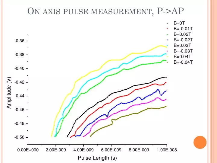
On axis pulse measurement, P->AP. On axis pulse measurement, P->AP. Extrapolated critical current. Extracted Coercive field 0.4T. DC critical current. Extracted Coercive field 0.4T. Dynamic Parameter. Lots of change over field range, however we do not have a line.

E N D
Extrapolated critical current Extracted Coercive field 0.4T
DC critical current Extracted Coercive field 0.4T
Dynamic Parameter Lots of change over field range, however we do not have a line
Extrapolated critical current Extracted Coercive field 0.25T
DC critical current Extracted Coercive field 0.1T
Dynamic Parameter Linear dependence of the applied field
Include dynamic parameter dependence on field in sun model The reversal will happen so long as the pulse pushed The magnetization so that the field can switch the magnetization by itself. • In the uniaxial case: This angle should be the one to use in the sun formulae to get our fitting parameters.
As long as Bz is small Problem: we are doing the case when switching angle is far from equilibrium, the linear model has already broken down.Anyway the correction is small (10%) not enough to get better agreement with the full calculation
Linearization of LLG equation near equator LLG Equation in the axially symmetric case Near the equator we can write And we get a new equation which we can try to approximate again
After linearization We can neglect the anisotropy term because it is small to the second order, and we get
What we want to do now is to separate the dynamics into two part that join at The time spent in the near-equilibrium regime should be much bigger hence:
As long as the spin torque is sufficiently high (Should be the case in the dynamic regime If we use the same argument for theta as before: Correction can be high, depending on
Simulation Results • Alpha=0.1 • Polarization=0.2 • Ms=713000 • Bc=0.1T • Initial angle=0.01rad • Vol=100x100x1.6 nm^3 • A parameter at 0field=1.61e11 (Vs)-1 • Original Sun formulae: 2e11 • Double model for theta1=0.1=>1.68e11
It is actually possible to fit simulation data to 10% accuracy with near 10degrees. • However we must justify the switch of the modelsWe could numerically compute the third order approximation around 0 or the second order around the equator and switch once first and higher order approximations differ by a significant amount.