Download
1 / 38
380 likes | 444 Views
Multi-wavelength SFR Tracers (an incomplete and biased summary). Daniela Calzetti (UMass), with a number of co-conspirators: R.C. Kennicutt (IoA, Cambridge U) Janice Lee (Carnegie Observatories) Rupali Chandar (UToledo) Alison Crocker (UMass) Yiming Li, Guilin Liu (UMass) + SINGS Team

E N D
Multi-wavelength SFR Tracers(an incomplete and biased summary) Daniela Calzetti (UMass), with a number of co-conspirators: R.C. Kennicutt (IoA, Cambridge U) Janice Lee (Carnegie Observatories) Rupali Chandar (UToledo) Alison Crocker (UMass) Yiming Li, Guilin Liu (UMass) + SINGS Team + LVL Team + WFC3 SOC (+, in the n-future, KINGFISH Team) UCL Colloquia, Cumberland Lodge, July 5-8, 2010
General Comment After the yoga class yesterday, I hope Mark W. realizes that he has raised my overall expectations for the quality of any future conference he will organize.
The Obligatory Big-Picture Slide AgeUniv= 13.5 3.23 1.52 0.92 Gyr Hopkins & Beacom 2006
Second Obligatory Big-Picture Slide: The Scaling Law(s) of SF In galaxies considered as a whole, the SFR scales with the gas surface density (Kennicutt 1989, Kennicutt 1998, Kennicutt 2006): SFR ~ gas1.4 Log SFR Log gas
Third Big-Picture Slide(Non-Obligatory) Kennicutt et al. 2007 Bigiel et al. 2008; Leroy et al. 2008 General agreement: HI has a `saturation’ limit Disagreement: slope of SSFR with SH2 : superlinear (~1.4) vs. linear/sublinear (~0.8-1)
What Does the Words `Star Formation Rate Tracers’ Imply: They imply that we know: How to convert a luminosity into a SFR (and, above all, that we understand what that luminosity is tracing); How to account for dust, in the form of both extinction and emission; How the stellar Initial Mass Function (IMF) behaves. A lot of the recent progress has been brought by Spitzer and GALEX, and Herschel promises to continue the legacy
SFR tracers Herschel Spitzer `calorimetric’ IR (m) 1 10 100 1000 24 m 70 m 160 m 8 m LMT/50 ALMA [OII] P H UV Dust-processed light Direct stellar light
M51, UV(GALEX)+H+24(Spitzer) What SFR are we tracing? C. et al. 2005; Rellano & Kennicutt 2009 UGC8201, UV(GALEX)+H+24(Spitzer)
An unsettling result… UGC8201, UV(GALEX)+H+24(Spitzer) (Lee et al. 2009, Meurer et al. 2009, Hoversten & Glazebrook 2008) How those galaxies look like:
Options: • All low luminosity galaxies are caught in a post-starburst phase (all of them?) or SF is sporadic/bursting (however, see mean SFH of dwarfs….) • Ionizing photons are diffused or leak out (unclear, hard to prove). • IMF varies as a function of some galaxy parameter (SFR, SFI, luminosity, etc.): • Most massive cluster a function of the SFR (Weidner, Kroupa & Larsen 2004); • Most massive star a function of the cluster’s mass (Weidner, Kroupa & Bonnell 2010).
SFH of Dwarf Galaxies Even the most metal-poor galaxies in the local Universe have stellar populations > 2 Gyr (Tosi 2009, and refs) SFH of dIs consistent with constant SF (Hunter et al. 1986+; Mateo 1998; Weisz et al. 2008) ~10% of stellar pops formed within past 1 Gyr (~30% within past 6 Gyr, Weisz et al. 2008) Birth-rate parameter ~ constant between low-mass and high-mass galaxies (Lee et al. 2007) I Zw 18
Options: • All low luminosity galaxies are caught in a post-starburst phase (all of them?) or SF is sporadic/bursting (however, see mean SFH of dwarfs….) • Ionizing photons are diffused or leak out (unclear, hard to prove). • IMF varies as a function of some galaxy parameter (SFR, SFI, luminosity, etc.): • Most massive cluster in a galaxy is a function of the SFR (Weidner, Kroupa & Larsen 2004); • Most massive star in a cluster is a function of the cluster’s mass (Weidner, Kroupa & Bonnell 2010). Hoversten & Glazebrook 2008, Lee et al. 2009
How do we test the cluster-star mass hypothesis? • Standard methods (star counts) are difficult/fail beyond the MCs, for massive stars. Too much blending. • Try to use star clusters (units of SF) themselves: • coeval SF; • Concentrate on young clusters (<=10 Myr), because massive stars die out in older clusters. M83, WFC3/ERS: U(blue), V+I(green), Ha(red)
Predictions for compact star clusters:are 100 clusters each 100 Mo equivalent to one 10,000 Mo cluster? • <Nion>/<Mcluster> produces very different trends as a function of Mcluster for: • Invariant IMF; • Weidner/Kroupa/Bonnell IMF model • Requirements: • Identify clusters (-> HST) • Measure ages and masses (5-6 photometric bands) • Measure Nion(narrow-band) • Average out SFHs and stochastic sampling (large, ~100, numbers of clusters) C., Chandar, Lee, Elmegreen, Kennicutt, Whitmore, 2010, ApJL, submitted Compare with Corbelli et al.’s `Birthline’
Initial Results: M51 High-end of IMF does not appear to change in low mass clusters, down to 103 Mo. Not the strongest test so far (need to go to lower mass clusters). Control of uncertainties/systematics is crucial (e.g., ionizing photon dispersion, etc.) On-going analysis of M83 and NGC4214; next step: very low SFR galaxies (when and if data become available)
In the meantime: how do I measure the SFR? UGC8201, UV(GALEX)+H+24(Spitzer) (Lee et al. 2009, Meurer et al. 2009, Hoversten & Glazebrook 2008) Maybe, the UV should be used (assuming we know how to control dust attenuation!).
M51, UV(GALEX)+H+24(Spitzer) Can I use the UV here, too? In other words, are regions within galaxies independent, for what concerns SFR tracers? C. et al. 2005; Rellano & Kennicutt 2009) Let’s recall that we translate stellar flux into a SFR
Let’s play a game: • Let’s focus on the UV emission around 1500 Angstrom (GALEX). • Let’s assume that we are interested on two timescales: 10 Myr (ionizing photons) and 100 Myr (UV flux). • Let’s assume SF is constant over the longest timescale and that we have a good way of correcting for dust attenuation. • How much UV flux is associated with the 0-10 Myr old population and how much with the population in the 10-100 Myr range? • If the stars have dispersion velocity ~10 km/s, how much ground will they have covered in 10 Myr? And in 100 Myr?
Model comparison: 100 Myr vs 10 Myr constant SF 100 Myr ~30% 10 Myr
Let’s play a game: • Let’s focus on the UV emission around 1500 Angstrom (GALEX). • Let’s assume that we are interested on two timescales: 10 Myr (ionizing photons) and 100 Myr (UV flux). • Let’s assume SF is constant over the longest timescale and that we have a good way of correcting for dust attenuation. • How much UV flux is associated with the 0-10 Myr old population and how much with the population in the 10-100 Myr range? • a: ~70% ; b: ~ 30% • If the stars have dispersion velocity ~10 km/s, how much ground will they have covered in 10 Myr? And in 100 Myr? • a: ~ 100 pc ; b: ~ 1 kpc
About 30% of the original UV light will be distributed over an area ~10x the area of the remaining 70% (streaming away from an arm) This happens for the SF both in the arm regions and the interarm regions. In M51, the observed (attenuation-corrected) arm/interarm UV ratio is ~15:1 ~2 kpc
Potential Impact of Population Mixing on SFR Measurements (UV) • If the MCs remain close to regions of most recent SF: • Removal of local bck will cause an underestimate of the intercept in the SK Law; • Non-removal of local bck will produce an artificial trend. • (This does not include another problem: the `extinction-corrected’ UV is obtained from IR emission, which is affected by `old-population’ heating)
Is this observed? It is observed, both in (ext-corr) UV and in Ha in two galaxies: M51 (depicted) and NGC3521. Local bck subtraction on the stellar pops is an essential portion of the measurement (already noted by Bigiel et al. 2008) Non-bck sub Bck-sub (Liu et al. in prep.)
Moving to Redder l: IR SFR tracers Herschel Spitzer `calorimetric’ IR (m) 1 10 100 1000 24 m 70 m 160 m 8 m LMT/50 ALMA [OII] P H UV Dust-processed light Direct stellar light The IR (integrated over SED) can be problematic: heating by `old’ stellar populations. Often SED-integrated IR is not available!
SFR(Mid-IR)PAH C. et al. 2007 Wu et al. 2005 ISO enabled the first studies aimed at investigating monochromatic IR emission as SFR tracer, specifically in the UIB=AFE=PAH bands (e.g., Madden 2000, Roussel et al. 2001, Boselli et al. 2004, Forster-Schreiber et al. 2004, Peeters et al. 2004, etc.) Spitzer continued the tradition… Alonso-Herrero et al. 2006
More calibrations…. Zhu et al. 2008 Kennicutt et al. 2009 Common features: 1. Linear or sligthly sub-linear correlation [The Perfect Calibrator?]; 2. Strong dependence on metallicity; 3. Possibly offset between HII regions and galaxies calibrations (diffuse emission) Log (Hacorr)
Dependence on Metallicity Draine et al 2007 Engelbracht et al. 2008 Effect not due to PAH ionization or de-hydrogenation effects (Smith et al. 2007). However, there may be PAH size variations (Smith et al. 2007, Hunt et al. 2010, Sandstrom et al. 2010). Boselli et al. 2004, Madden et al. 2006, Engelbracht et al. 2005, Hogg et al. 2005,Galliano et al. 2005,2008, Rosenberg et al. 2006, Wu et al. 2006, Munoz-Mateos et al. 2009, Marble et al. 2010 Smith et al. 2007
Nature (PAH Formation) or Nurture (PAH Processing)? (Gordon et al. 2008) Better correlation with ionization index (a combination of [NeIII]/[NeII] and [SIV]/[SIII] ratios], than with metallicity (M101 and starbursts). Low-met galaxies characterized by hard radiation fields(Hunt et al. 2010) (Cesarsky et al. 2000, Madden et al. 2006,Wu et al. 2006, Bendo et al. 2006, Berne’ et al. 2007, Smith et al. 2007, Gordon et al. 2008, Engelbracht et al. 2008)
How to Quantify Diffuse PAH -1 • Mask out clustered regions of star formation (HII regions/clusters) • Separate diffuse PAH associated with diffuse ionizing photons from `other’ diffuse PAH emission (Crocker et al., in prep.)
How to Quantify Diffuse PAH -2 • Preliminary results for NGC628: • Diffuse PAH emission fraction • ~ 20-30% of total (once extinction corrections are included) • ratio highly dependent on • galactocentric distance • (about twice more diffuse • PAH emission in the • outskirts than in the central • areas. • Preliminary result! • (approximately corrected • for dust extinction) Without ext-corr (Crocker et al., in prep)
A Robust Measure of SFR L(H) = unobscured SF; L(24m) = dust-obscured SF a L(H)+b L(24 m) HII regions+starbursts Normal SF Galaxies Galaxies: SFR (Mo yr-1) = 5.45 x 10-42 [L H, obs + 0.020 L24m (erg s-1)] L(24)<4 X 1042 = 5.45 x 10-42 [L H, obs + 0.031 L24m (erg s-1)] = 1.70 x 10-43 L24m [2.03 x 10-44 L24m]0.048 L(24)>5 X 1043 Kennicutt et al. 2007, 2009; C. et al. 2007, 2010
SFR(70) Mostly linear…. HII regions/complexes Log[L(70)] Whole galaxies Log(SFR) Y. Li et al. 2010, submitted Calibration constant is a factor 60% higher than in the case of whole galaxies. Non-SF populations contamination? Repeat the analysis with Herschel+HST data (KINGFISH project)!
KINGFISH: The TEAM UK: Rob Kennicutt (PI), Paul Alexander, Dave Green, Ben Johnson, John Richer U.S.A.: Daniela Calzetti (Deputy PI), Phil Appleton, Lee Armus, Pedro Beirao, Alberto Bolatto, Alison Crocker, Kevin Croxall, Danny Dale, Bruce Draine, Chad Engelbracht, Karl Gordon, Joannah Hinz, Jin Koda, Adam Leroy, Eric Murphy, Nurur Rahman, Ramin Skibba, JD Smith, Mark Wolfire France: Helene Roussel, Marc Sauvage, Sundar Srinivasan, Laurent Vigroux Germany: Oliver Krause, Sharon Meidt, Hans-Walter Rix, Karin Sandstrom, Eva Schinnerer, Fabian Walter Italy: Leslie Hunt Netherlands: Bernhard Brandl, Brent Groves Spain: Amando Gil de Paz Canada: Christine Wilson, Brad Warren China: Caina Hao
Main Science Goals • Mapping of dust emission at peak energy over ~300-500 pc scales, combined with UV/optical/IR(Spitzer) images: • Spatially-resolved dust temperature distributions and masses; improved modeling; correlations between heaters (stellar populations) and emitters (dust conmponents); • Calibration of SFR diagnostics on sub-kpc scale; accurate determinations of the SFR-gas densities relation and SFR thresholds; • Sub-kpc radio-FIR correlation; • Full inventory of cold (< 15 K) dust • PACS spectroscopy of main ISM cooling lines to map temperatures, densities, pressures, local UV radiation strenght and hardness: • Investigate range of physical conditions of the ISM • [CII] and other lines as SFR indicators; • Solve the discrepancy in the metal abundance scale.
NGC1097 SBb D=19.1 Mpc PACS 70/100/160 Optical
M101 SABcd D=7.1 Mpc SPIRE 250/350/500 Optical
Summary and Conclusions • Standing issues for all SFR indicators: • IMF variations (may not be an actual variation; it may be a `sorted universality’) • Clustered vs. diffuse emission in spatially-resolved studies, and the problem of stellar population mixing. • Overall progress in all areas (i.e., at all wavelengths) of SFR calibrations has been enabled by the combination of Spitzer and GALEX • IR monochromatic indicators (both global and local) • SFR(8 mm) strongly depends on metallicity (physical origin, either nature or nurture, still debated) • SFR(24 mm), SFR(70 mm) or combinations less strongly dependent • Offsets in calibration constants between global and local SFR indicators suggest non-negligible diffuse component • Caveats: AGNs, range of applicability,