Download
1 / 15
150 likes | 249 Views
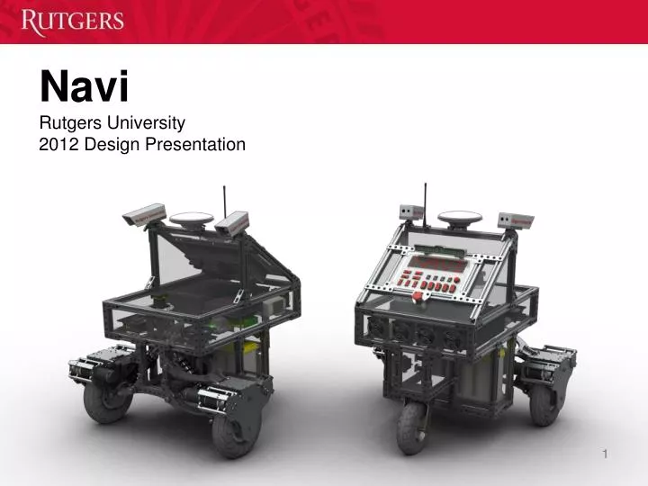
Navi Rutgers University 2012 Design Presentation. Mechanical Design. Entirely custom chassis Designed using SolidWorks 80/20 a luminum framing 0.25” polycarbonate casing 240 lb , including payload Brushed DC drive motors 80 W, 500 CPR optical encoders 5.6 mph maximum speed

E N D
Mechanical Design • Entirely custom chassis • Designed using SolidWorks • 80/20 aluminum framing • 0.25” polycarbonate casing • 240 lb, including payload • Brushed DC drive motors • 80 W, 500 CPR optical encoders • 5.6 mph maximum speed • 27% maximum grade • Actively air cooled by six fans • 100 cfm airflow through chassis • Modeled using CFD simulation
Electrical: Power Distribution • Optima YellowTop Battery (×2) • 12 V lead acid batteries (in series) • 35 A·h capacity • Low power consumption • 400 W loaded, 215 W idle • 2+ hour battery life • 24 V, 12 V, and 5 V DC buses • 85%+ efficiency DC-DC regulators • Isolated grounds limit noise • Dashboard • Switches for major components • Dot matrix display status indicator
Software Architecture • Use and contribute to open source software when possible • Built on the Robot Operating System (ROS) framework • Three-dimensional Gazebo simulation of driving and sensors Localization Planning Gazebo Gazebo Perception
Localization: Sensors GPS: Novatel ProPak V3 • 2 Hz sample rate • 15 cm accuracy (1 sigma) • OmniSTAR HP corrections Compass: PNI Fieldforce TCM • 50 Hz sample rate • 0.3° heading accuracy (RMS) • 360° tilt correction Odometry: US Digital Encoders • 500 CPR, 0.5 mm resolution
Localization: Extended Kalman Filter • Fuse sensors to estimate pose • Odometry: fast, relativepose • Compass: fast absolute orientation • GPS: accurate absolute position • Non-linear “turn-drive-turn” model (Source: Probabilistic Robotics) Simulation Hardware
Perception: Sensors Laser: Hokuyo UTM-30LX • 40 Hz sample rate • 240° field of view • 30 m maximum range Cameras: AVT Manta G-125C (×2) • 15 FPS, synchronized • 646 × 482 resolution • 90° × 65° wide angle lens • 130° combined field of view
Perception: Sensors Laser: Hokuyo UTM-30LX • 40 Hz sample rate • 240° field of view • 30 m maximum range Cameras: AVT Manta G-125C (×2) • 15 FPS, synchronized • 646 × 482 resolution • 90° × 65° wide angle lens • 130° combined field of view
Perception: Line Detection • Uses the HSV color space to limit the impact of illumination • Width filter is generated from the calibrated camera matrix • Pipelined with left and right images processed in parallel • Total processing time is 100 msper image pair • Pipelining allows for a 50% increase in sample rate Width Filter Color Transformation Original Image
Mapping Local Costmap: (10 m)2 • 5 cm square cells; high resolution • Always centered on the robot • Used by the local planner Global Costmap: (1000 m)2 • 25 cm square cells; low resolution • Origin fixed by a GPS coordinate • Used by the global planner • Sensors mark and clear observations • Based on the ROS navigation stack
Planning Global Planner (on demand) • Weighted A* Search • Inverse of distance for <1 m • Constant for ≥1 m Local Planner (20 Hz) • Dynamic Window Approach • 10 linear velocity samples • 15 angular velocity samples