Download
1 / 18
180 likes | 320 Views
Magnetospheric Modeling. M. Wiltberger and E. J. Rigler NCAR/HAO. Outline. What is the magnetosphere? How do we model it? Possible areas where statistics can help us. Solar Origins. Solar Flares - abrupt release of energy localized solar region mainly radiation (UV, X-rays, γ -rays)

E N D
Magnetospheric Modeling M. Wiltberger and E. J. Rigler NCAR/HAO
Outline • What is the magnetosphere? • How do we model it? • Possible areas where statistics can help us
Solar Origins • Solar Flares - abrupt release of energy • localized solar region • mainly radiation (UV, X-rays,γ-rays) • occur near complex sunspot configurations • Coronal Mass Ejections (CMEs) • Releases of massive amounts of solar material • Usually with higher speeds and greater magnetic fields than surrounding solar wind • Usually cause shocks in solar wind • Solar Wind • Steady ionized gas outflow with average velocity 400 km/s • Magnetic field direction variable • Exact properties depend upon solar origins
Earth's Magnetosphere • The magnetosphere is region near the Earth where it's magnetic field forms a protective bubble which impedes the transfer of energy and momentum from the solar wind plasma • A variety of different phenomenon • Substorms • impulsive energy release over hours • Storms • globally enhanced activity over days • Radiation belts • trapped particles which are omnipresent
Dayside and R1 Currents Neutral Sheet Current Ring and R2 Currents Magnetospheric Currents • Magnetopause current systems are created by the force balance between the Earth’s dipole and the incoming solar wind
Ionospheric Currents • FAC from the magnetosphere close though Pedersen and Hall Currents in the ionosphere Region 1 Region 2
LFM Magnetospheric Model • Uses the ideal MHD equations to model the interaction between the solar wind, magnetosphere, and ionosphere • Computational domain • 30 RE < x < -300 RE & ±100RE for YZ • Inner radius at 2 RE • Calculates • full MHD state vector everywhere within computational domain • Requires • Solar wind MHD state vector along outer boundary • Empirical model for determining energy flux of precipitating electrons • Cross polar cap potential pattern in high latitude region which is used to determine boundary condition on flow
Computational Grid of the LFM • Distorted spherical mesh • Places optimal resolution in regions of a priori interest • Logically rectangular nature allows for easy code development • Yee type grid • Magnetic fluxes on faces • Electric fields on edges • GuaranteesB = 0
Ionosphere Model • 2D Electrostatic Model • (P+H)=J|| • =0 at low latitude boundary of ionosphere • Conductivity Models • Solar EUV ionization • Creates day/night and winter/summer asymmetries • Auroral Precipitation • Empirical determination of energetic electron precipitation
Calculation of Particle Fluxes • Empirical relationships are used to convert MHD parameters into an average energy and flux of the precipitating electrons • Initial flux and energy (Fedder et al., [1995]) • Parallel Potential drops (Knight [1972], Chiu [1981]) • Effects of geomagnetic field (Orens and Fedder [1978])
Determining Energy Flux • According to Lummerzheim [1997], it is possible using the UVI instrument on POLAR to determine both the characteristic energy and energy flux • Energy flux is proportional to emission rates in the LBH bands • Characteristic energy determines altitude of emission so it is determined by monitoring brightness of features that decay away and those that persist
Estimating Optimal Parameters • LFM electron flux/energy estimates are projected onto irregular grid corresponding to Polar UVI observations: • 1-D “state vector” constructed from all available observations; time is simply treated as a third coordinate, in addition to MLT and ALAT; • Levenberg-Marquardt (nonlinear least-squares) algorithm adjusts model parameters a, b, and R to minimize the sum of the squared prediction errors:
Can advanced statistics help us? • Are there better parameter estimation algorithms then Levenberg-Marquart? • What can statistical comparisons with observations tell us about the bias present in our models? • What are the best measures to monitor model improvement over time?
Some Research Problems 1. How can uncertain model parameters be optimized to provide the best agreement, on the average, with observations? 2. How can model variability about the average, including information about scale sizes of this variability, best be compared with variability in observations to determine agreement or disagreement? 3. How can we improve the interpolation/extrapolation of observations of model input parameters in space and time to get complete specification of the boundary conditions? 4. In developing parameterizations of sub-grid phenomena, such as the transport of momentum and the creation of turbulence by breaking gravity waves, what is a good measure of intermittency, and how can its effects be parameterized? 5. How can relatively rare and sparse observations of extreme events like large magnetic storms be used to characterize upper-atmospheric behavior and test simulations for such events? 6. What can statistical comparisons tell us about underlying biases in our models? 7. What are the best measures to monitor model improvement over time?
MI Coupling Eqs • As described in Kelley [1989] The fundamental equation for MI coupling is obtain by breaking the ionospheric current into parallel and perpendicular components and requiring continuity • Assuming no current flows out the bottom of the ionosphere we get • Further assuming the electric field is uniform with height we get • And finally using and electrostatic approximation in the MI coupling region we obtain
Hardy et al. [1987] reports a version of the Robinson et al. with slight typographical error Conductances from Particle Flux • Spiro et al. [1982] used Atmospheric Explorer observations to determine a set of empirical relationships between the average electron energy and the electron energy flux • Robinson et al. [1987] revised the relationships using Hilat data and careful consideration of Maxwellian used to determine the average energy