Loss-Bounded Analysis for Differentiated Services.

1. Loss-Bounded Analysis for Differentiated Services. By Alexander Kesselman and Yishay Mansour Presented By Sharon Lubasz 042824821

2. Abstract • Network Service offering different levels of Quality of Service (QoS). Only trivial bounds could be obtained by traditional competitive analysis. Introduction of a new approach called Loss-Bounded analysis. Derive tight upper and lower bounds for various settings of the new model.

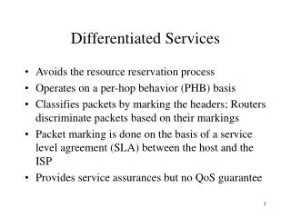
3. Introduction In the Differentiated Services priority model: packets of different QoS priority have distinct benefit values: The lowest benefit of 1. • The highest benefit denoted α , α≥1. • For advanced traffic models, there maybe a need for more than two distinct benefits. Basic Paradigms: Research of differentiated services For internet traffic products two basics paradigms: The premium service. The assorted service.

4. Basic Paradigms (cont.) The premium service model: The premium service model provides the same QoS guarantee as a dedicated line, with a predefined bit rate. A premium service traffic is shaped at the entry to the network; hard limited to its provisioned peak rate. The assorted service model: The assorted service model traffic flow may exceed its provisioned rate. The excess traffic is not given the same assurance, if any. The FIFO buffering policy : Most of today’s internet routers work with FIFO buffering policy. Critical for many application. Simplifies and enable to achieve efficient hardware implementation. Reflects the the nature of the network- the main internet protocol is TCP- optimized in FIFO order.

5. The Model A single FIFO queue. Serves online - without knowledge of future packets. Performs two functions: 1. Stores. 2. Selectively rejects/preempts packets subject to the buffer. The goal: to maximize the policy’s benefit. Definitions: For a sequence of packets S and an online policy A we denote: • The subsequence of packets with benefit B, denoted Sb. • The entire benefit of the sequence denoted V(S) =∑pєS b(p). • The benefit of A on S, denoted VA(S) And the loss of A on S, denoted LA(S) . • V(S) = VA(S) + LA(S) . • Denoted the optimal offline policy by OPT. VOPT(S) the optimal benefit. LOPT(S) the optimal loss.

6. Competitive Analysis The online policy is compared with an optimal offline policy that knows the input in advance. Throughput Competitive and Loss Competitive Throughput Competitive An online policy A, is said to be C-Throughput Competitive if for any input sequence, its benefit constitutes at least a C fraction of the benefit of an optimal offline policy. A is C-throughput Competitive iff for every sequence of packets S, VA(S) ≥ C  VOPT(S) . Loss Competitive An online policy A, is said to be C-Loss Competitive if the loss of an optimal offline policy constitute at least a C fraction of its loss. A is C-Loss Competitive iff for every sequence of packets S, LOPT(S) ≥ C  LA(S) . A Throughput Competitive guarantee ≠> Loss Competitive guarantee.

7. Motivation and Loss-Bounded Loss-Competitive guarantee is much more desirable then Throughput Competitive. Unfortunately, only trivial bounds can be obtained by it. Motivated by this, we propose a new model, called Loss-Bounded Analysis, for estimating loss of an online policy. Loss-Bounded Analysis In C-Loss-Bounded Analysis, the loss of an online policy is upper bounded by the loss of the optimal offline policy plus a C fraction of the benefit of the optimal offline policy. We let this fraction C be the Loss-Bounded ratio of the online policy. • Loss-Bounded Analysis provides Throughput Competitive guarantee. One can either maximize the throughput of the policy or minimize its loss. • An optimal solution to one problem do not necessarily lead to a good approximation of the other.

8. Loss-Bounded Analysis andSome Intuition The intuition behind Loss-Bounded Analysis is that we try to optimize both parameters simultaneously, by finding an optimal tradeoff between the current gain and the potential loss. Definition: A is C-Loss-Bounded iff for every sequence of packets S, LA(S) ≤ LOPT(S) + C  VOPT(S) . The Model - Additions The FIFO buffer can hold B packets. Packets may arrive at any time. Send events are synchronized with time. The system obtains the benefit of the packets it sends. Aiming to maximize the benefit. When a packets arrives, a queuing policy can either reject or except it. • Each time unit, a send operation is executed on the first packets in the buffer (first in queue).

9. The Scheduling Policy An arriving packet is accepted if either the buffer is not full or that the buffer is full, and a minimal benefit among the packets in the buffer is less then the benefit of the arriving packet. In that case, a packet with minimal benefit is preempted from the buffer before acceptance of the arriving packet. β-Preemptive Greedy Policy Behaves like a greedy policy, except, that upon acceptance of a packet, βadditional packets may be preempted. The preempted packets are the low-benefit packets closest to the transmitting end of the FIFO queue buffer. Definition: Overloaded Scheduling Interval • Some high benefit packets where rejected during the interval. • The longest time interval during which only high benefit packets were sent.

10. Binary Benefit Values THEOREMThe greedy policy is 1/α Loss-Competitive. Proof.By definition, the cumulative benefit of the lost packets is at most far by a factor of α from the optimal. …for the next Theorem we will need some more tools... Auxiliary Lemmas and Claims LEMMAWhen packets are scheduled according to the √α - preemptive greedy policy, and there are at least B/√α high benefit packets in the buffer, then at the next time unit, a high benefit packet will be sent. Proof.There can be B low benefit packets at most (the whole buffer). We know that there are B/√α high benefit packets, so for eachB/√α packets √α low benefit packets are preempted… that is the whole B low benefit packets… And so, the only packets left to send are high benefit ones.

11. Auxiliary Lemmas and Claims (cont.) CLAIMWhen packets are scheduled according to the √α - preemptive greedy policy, the number of high benefit packets in the buffer at the time unit preceding the beginning of an overloaded interval [ts ,tf ], is at most B/√α. Proof.There can be two cases: 1. If the queue was empty at the the beginning of the interval, then clearly there where less then B/√α high benefit packets. • The interval started after a low benefit packet was sent (time unit ts-1). Lets assume that at time ts-2 there are B/√α or more high benefit packets, then by the lemma a low benefit packet couldn’t have been sent at ts-1. So, it is guaranteed that at ts-2 there are at the most (B/√α)-1 high benefit packets. And so, it is guaranteed that at ts-1 there are at the most (B/√α) high benefit packets.

12. Auxiliary Lemmas and Claims (cont.) and More Theorems CLAIMWhen packets are scheduled according to the √α–Preemptive Greedy Policy the length of an overloaded interval is at least B. Proof.By definition during the interval at least one high benefit packet must be lost, that could have occurred only when the buffer was full of other high benefit packets. At least those B packets will be send. THEOREMThe Loss-Bounded ratio of the greedy policy is at most (α-1)/α and at least(α-1)/2α. More Theorems Proof.In the worst case scenario, A benefits at leastVOPT(S)/α, of the optimal gain. And so A losses the maximum possible minus what A gains: VOPT(S) – (VOPT(S)/α) = (1-1/α)VOPT(S) LA(S) ≤ LOPT(S) +(1-1/ α)VOPT(S) = LOPT(S)+((α-1)/ α)VOPT(S)

13. More Theorems (cont.) • This is the worst case scenario in which A sends a low benefit packet (benefit of 1) for every packet that the offline • optimal policy sends a high benefit packet (benefit of α). More intuition for the upper bound: For the lower bound, lets look at the worst case scenario: • A burst of B low benefit packets. • For B time units every time units a high benefit packet arrives. • A burst of B high benefit packets. The Greedy policy: Receives the burst and enters the packets to the buffer. In queues a high benefit packet and transmits the low benefit packets from the head of the buffer. Ignores the burst of the high benefit packets as the buffer is full with high benefit packets. LA(S) = Bα…the loss of the last high benefit burst.

14. LOPT(S)=B…the loss of the low benefit burst. VOPT(S)=2Bα. More Theorems (cont.) page 2 The optimal policy: Ignores the low benefit burst. Receives and sends the high benefit packets one by one. Receives the high benefit burst. Bα≤ B + C (2Bα). => by definition C = (α –1)/2(α) =>

15. More Theorems (cont.) page 3 THEOREMThe Loss-Bounded ratio of the √α-Preemptive Greedy policy is at most 2/√α . Proof.We process the loss of low benefit packet, denoted S1, and loss of high benefit packets, denotes Sα, separately. First we bound the loss of the low benefit packet. Their are two kinds of losses of low benefit packets: • A loss of a low benefit packet due to additional preemptions (a high benefit packet arrives while the buffer was full) denote LAextra. • A loss of a low benefit packet due to buffer overflow. denote LAovfl. LA(S1) = LAextra(S1) + LAovfl(S1)

16. LA(S1) ≤(1/√α)VA(Sα)+ LAovfl(S1) LA(S1) = LAextra(S1) + LAovfl(S1) More Theorems (cont.) page 4 First case: Denote S’α all the high benefit packets that caused the preemption of a low benefit packet. Note that S’α C Sα.– VA(S’α) = ( ( LAextra(S1) ) / √α ) α The benefit on all the packets that were received after preempting low benefit packets. The number of high benefit packet that was received after preempting low benefit packets. LAextra(S1) = (VA(S’α)√α)/α = (1/√α)VA(S’A) ≤ (1/√α)VA(Sα) => => LAextra(S1) ≤(1/√α)VA(Sα). Second case: The number of low benefit packets that are lost due to the buffer’scapacity constrains - overflow - can be bounded the number of packetsthat are lost by an optimal offline policy, The constrains are due to the buffer topology, and so the optimal policy will also be affected by it. => LAovfl(S1)≤LOPT(S1). LA(S1) ≤ (1/√α)VA(Sα)+LOPT(S1).

17. => LA(Sα) ≤ LAadd(Sα) + LOPT(Sα) . Clearly, LA(Sα) = LAadd(Sα) + LAncs(Sα) . More Theorems (cont.) page 5 High benefit packets can be lost due to lack of space in the buffer, just like an optimal offline policy, denote this lossLAncs. LAncs(Sα) ≤LOPT(Sα). As shown at the beginning of overloaded interval there are at most B/√αhigh benefit packets in the buffer. An optimal offline policy could have send these additional packets. If A were to throw this packets hewould have simulated the optimaloffline policy. DenotedLAadd(Sα). As shown the length of an overloaded interval is at least B, and so the ratiobetween the loss and the cumulative benefit of the packets scheduled during anoverloaded interval is at most: B√α/ Bα = 1/√α ≥ LAadd(Sα) / VA(Sα) the upper bound on the loss of LAadd The lower bound on the benefit of A. LAadd(Sα) ≤ (1/√α)VA(Sα). LA(Sα) ≤ (1/√α)VA(Sα)+LOPT(Sα) .

18. + =========================== LA(S) ≤ (2/√α)VA(S)+ LOPT(S) Summary Lets sum up: LA(S1) ≤ (1/√α)VA(Sα)+ LOPT(S1) LA(Sα) ≤ (1/√α)VA(Sα)+ LOPT(Sα) Binary Benefit Values Setting Results 1/α (α-1)/α Greedy √α-Prmpt. Greedy 0 2/√α As shown the greedy policy achieves 1/α Loss-Competitive ratio which is the tight upper bound. Thus, the bound for the √α- Preemptive Greedy Policy approaches 0 when α is large.

19. We extension of the two benefit model to the case of n different values: {αi/n: 0 ≤ i ≤ n} 1/α (α-1)/(α+1) Greedy (n+2)/√(α1/n) + 2/α1/n √(αi/n)-Prmpt.Greedy 0 1/α 1/2√(α1/n) Impossibility Results Extended Models All the results of the Loss-Competitive Analysis are trivially extended to the Restricted and Arbitrary benefit models. Restricted Benefit Model Restricted Benefit Values Setting Results !!! As the number of values increases the guarantee is weakened. !!!

20. 1/α (α-1)/(α+1) Greedy 1/α Impossibility Results 1/8logα Arbitrary benefit Model We extend the n benefit model to arbitrary benefit model so that for any packet its benefit is between 1 and α. Arbitrary Benefit Values Setting Results No online policy under arbitrary benefit values model can have less than logarithmic Loss-Bounded ratio. Due to the logarithmic ratio that cannot be better than 1/8logα, which is obviously bigger in a scale than the restricted polynomial bound of 2/√α, arbitrary benefit model is usually inefficient.

21. Concluding Remarks • Importance of analysis of the loss of an online policy. • The impossibility results for traditional competitive analysis. • Tight lower and upper bounds for FIFO buffer management and packets scheduling. • Loss-Bounded Analysis can give much better performances then traditional Competitive Analysis. • The model provides simplicity which allows operation at very high speed and without additional equipment. • Operator can manage traffic streams in the best way by choosing the appropriate benefit setting.