Download
1 / 23
230 likes | 289 Views
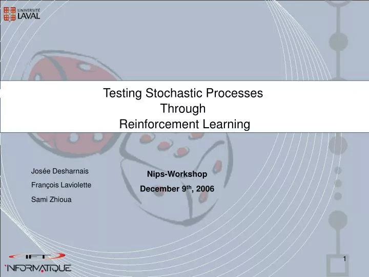
Testing Stochastic Processes Through Reinforcement Learning. Josée Desharnais. Nips-Workshop December 9 th , 2006. François Laviolette. Sami Zhioua. Outline. Program Verification Problem. The Approach for trace-equivalence. Other equivalences. Application on MDPs.

E N D
Testing Stochastic Processes Through Reinforcement Learning Josée Desharnais Nips-Workshop December 9th, 2006 François Laviolette Sami Zhioua
Outline Program Verification Problem The Approach for trace-equivalence Other equivalences Application on MDPs Conclusion
Stochastic Program Verification Specification (LMP): an MDP without rewards Implementation s0 a[0.3] a[0.5] s1 s2 b[0.9] c b[0.9] s4 s5 s3 c s6 The Specification model is available. The Implementation is available only for interaction (no model). How far the Implementation is from the Specification ? (Distance or divergence)
Q P b a a c c b a a c a a c a b c b b b b c b c a P a[1/3] b[2/3] a[1/4] a[1/4] a[2/3] c a[3/4] b c b[1/2] c[1/2] 2. Probabilistic trace equivalence a Q Two systems are trace equivalent iff they accept the same set of traces and with the same probabilities a[1/2] a[1/2] b aa 5/12 a[1/4] a[1/3] c a[3/4] b b[1/2] b[1/2] c a 7/12 a 1 a aa 1/2 bc 2/3 aac 0 … … aac 1/6 bc 0 Trace Equivalence 1. Non deterministic trace equivalence Two systems are trace equivalent iff they accept the same set of traces T(P) = {a, aa, aac, ac, b, ba, bab, c, cb,cc} T(Q) = {a, ab, ac, abc, abca, ba, bab, c, ca}
z a b The button goes down (transition) When a button is pushed (action execution) The button does not go down (no transition) Grammar (trace equiv): t ::= | a.t Observations : When a test is executed, several observations are possible : Ot. s0 Example: a[0.5] a[0.2] [2,4) [7,10] 0.3 0.56 0.14 b[0.7] s3 Testing (Trace Equivalence) The system is a black box. t = a.b. Ot = {a, a.b, a.b}
Outline Program Verification Problem The Approach for trace-equivalence Other equivalences Application on MDPs Conclusion
Why Reinforcement Learning ? MDP s0 LMP s0 a b b[0.9] 0.2 0.9 0.5 a[0.5] a[0.2] s1 s2 s3 s1 s2 s3 a a[0.3] a a b[0.7] b s5 s6 s4 1 0.7 0.3 s6 s4 s5 b a[0.7] s8 s7 b a 0.7 1 s7 s8 Reinforcement Learning is particularly efficient in the absence of the full model. Reinforcement Learning can deal with bigger systems. Analogy : MDP LMP Policy Trace Optimal Value ( V* ) Divergence
Specification Specification (clone) Implementation s0 s0 s0 a[0.5] a[0.2] a[0.3] b[0.9] a[0.3] b[0.9] a[0.2] a[0.2] s1 s1 s1 s2 s2 s2 a b[0.3] a b[0.3] a b[0.3] b[0.7] b[0.7] b[0.7] s4 s5 s4 s5 s4 s5 s3 s3 s3 c[0.8] c[0.8] b b b c[0.4] c[0.2] c[0.7] c[0.7] s8 s8 s8 s6 s7 s7 s9 s7 s9 b b b s10 s10 s10 F S S F S F F F S + 1 - 1 S F F S F S S S F 0 S S S F F F A Stochastic Game towards RL Reward : (+1) when Impl Spec Reward : (-1) when Spec Clone
s0 a b 0.2 0.9 0.5 s1 s2 s3 a b 1 0.3 0.7 s4 s3 s5 b c c 0.7 1 0.8 s8 s9 s7 b 1 s10 MDP Defintion MDP : Specification LMP States Actions Next-state probability distribution Spécification MDP Implémentation s0 s0 a[0.5] a[0.2] a[0.5] b[0.9] a[0.2] s1 s1 s2 s2 Dead a b[0.3] a b[0.3] b[0.7] b[0.7] s4 s5 s4 s5 s3 s3 c[0.8] b b c[0.4] c[0.2] c[0.7] s8 s8 s6 s7 s7 s9 b b s10 s10
Specification MDP Implementation s0 s0 Dead a[0.5] a[0.2] a[0.5] b[0.9] a[0.2] s1 s1 s2 s2 a b[0.3] a b[0.3] b[0.7] b[0.7] s4 s5 s4 s5 s3 s3 c[0.8] s0 b b c[0.4] c[0.2] c[0.7] s8 s8 s6 s7 s7 s9 a b b b 0.2 0.9 0.5 s10 s10 s1 s2 s3 a b 1 0.3 0.7 s4 s3 s5 b c c 0.7 1 0.8 F S S F F S s8 s9 s7 + 1 - 1 S F F S S F b F S F 1 S F S s10 0 S S S F F F Divergence Computation 0 : Equivalent V*(s0) 1 : Different *
Success variant ( a ) Create two variants for each action (a): Failure variant ( a ) Prediction: Compute and give reward If pred = obs execute action make a prediction (, ×) Select action If pred obs Give reward 0 Symmetry Problem Spec (Clone) Specification Implementation s0 s0 s0 a[1] a[0.5] a[0.5] s1 s1 s1 F S S F F S + 1 - 1 S F F S S F Prob=0*.5*.5+1*.5*.5 = .25 Prob=0*.5*.5+1*.5*.5 = .25
The Divergence (with the symmetry problem fixed) Theorem. Let "Spec" and "Impl" be two LMPs, and M their induced MDP. V*(s0) ≥ 0, and V*(s0) = 0 iff "Spec" and "Impl" are trace-equivalent.
Implementation and PAC Guaranty Implementation : RL algorithm : Q-Learning Action selection : softmax ( decreasing from 0.8 to 0.01) = 0.8 decreasing according to the function 1/x PAC guaranty : There exists a PAC Guaranty for Q-Learning Algorithm but .. Fiechter algorithm has a simpler PAC guaranty. Besides, it is possible to obtain a bottom bound thanks to the Hoeffding inequality : If then :
Outline Program Verification Problem The Approach for trace-equivalence Other equivalences Application on MDPs Conclusion
a b z Replication Grammar t ::= | a.t s0 Example: a[0.5] a[0.2] [2,4) [7,10] 0.518 0.098 0.042 0.3 0.042 b[0.7] s3 Testing (Bisimulation) The system is a black box. (bisimulation) : | (t1, … , tn) t = a.(b,b) Ot = {a, a.(b, b), a.(b,b), a.(b,b), a.(b,b)} Pt,s0 :
Q P c c a[1/3] a[2/3] a b[1/3] c[2/3] b c New Equivalence Notion ‘’By-Level Equivalence’’
Two systems are “By-level’’ equivalent is equal to k 1-moment (trace) 2-moment t ::= | ak.t k 2 3-moment t ::= | ak.t k 3 K-Moment Equivalence : is a random variable suchthat is the probability to perform the trace and make a transition to a state that accepts action a with probability pi . Recall : kth moment of X = E(Xk) = ( xik . Pr(X=xi)) t ::= | a.t
Q P a[1/2] a[1/2] a[1/3] a[2/3] b b a[1/4] a[1/3] c a[1/4] a[1/3] c a[3/4] b a[3/4] b c b[1/2] b[1/2] b[1/2] b[1/2] c a a 1. Failure Equivalence Q P Two systems are Ready equivalent iff for any trace tr and any set of actions A, they have the same probability to run successfully tr and reach a process refusing all actions from A. a[1/2] a[1/2] a[1/3] a[2/3] b b a[1/4] a[1/3] c a[1/4] a[1/3] c a[3/4] b a[3/4] b c b[1/2] b[1/2] b[1/2] b[1/2] c a a (<a>,{b,c}) 1/3 (<a>,{b,c}) 1/2 Ready Equivalence and Failure equivalence 1. Ready Equivalence Two systems are Ready equivalent iff for any trace tr and any set of actions A, they have the same probability to run successfully tr and reach a process accepting all actions from A. . (<a>,{b,c}) 2/3 (<a>,{b,c}) 1/2 Test t ::= | a.t | {a1, .. , an} Test t ::= | a.t | {a1, .. , an}
Q P a[1/2] a[1/2] a[1/3] a[2/3] b b a[1/4] a[1/3] c a[1/4] a[1/3] c a[3/4] b a[3/4] b c b[1/2] b[1/2] b[1/2] b[1/2] c a a Q P a[1/2] a[1/2] a[1/3] a[2/3] b b a[1/4] a[1/3] c a[1/4] a[1/3] c a[3/4] b a[3/4] b c b[1/2] b[1/2] b[1/2] b[1/2] c a a Barb equivalence 1. Barb acceptation Test t ::= | a.t | {a1, .. , an}a.t (<a,b>,<{a,b},{b,c},>) 2/3 2. Barb Refusal Test t ::= | a.t | {a1, .. , an}a.t (<a,b>,<{b,c},{b,c}>) 1/3
Outline Program Verification Problem The Approach for trace-equivalence Other equivalences Application on MDPs Conclusion
s0 r2 r3 r1 a b 0.2 0.9 0.5 s1 s2 s3 r3 r4 r5 a a b s0 1 0.7 0.3 s6 s4 s5 r2 r3 r1 a b 0.2 1 0.8 r7 r8 b a s1 s2 s3 0.7 1 s7 s8 r3 r4 r5 a b 1 0.3 0.7 Case 1 : The reward space contains 2 values (binary) : 0 and 1 s4 s3 s5 r6 r7 r8 Case 2 : The reward space is small (discrete) : {r1, r2, r3, r4, r5} b c c 1 1 1 Case 3 : The reward space is very large (continuous) : w.l.o.g. [0,1] s8 s9 s7 MDP 1 Application on MDPs MDP 2
Case 1 : The reward space contains 2 values (binary) F r1 : 0 S r2 : 1 Case 2 : The reward space is small (discrete) {r1, r2, r3, r4, r5} F r1 r2 r3 r4 r5 a a a a a S r1 r2 r3 r4 r5 b b b b b Case 3 : The reward space is very large (continuous) S ranVal r pick a reward value (ranVal) randomly a r F ranVal< r Application on MDPs 1 with probability 3/4 r = 3/4 Intuition : 0 with probability 1/4
Current and Future Work Application to different equivalence notions : • Failure equivalence • Ready equivalence • Barb equivalence, etc. Studying the properties of the divergence Experimental analysis on realistic systems Applying the approach to compute the divergence between : - HMMs - POMDPs - Probabilistic automata