1 / 60

E N D
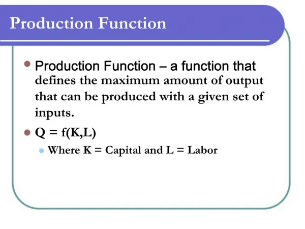
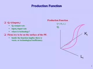
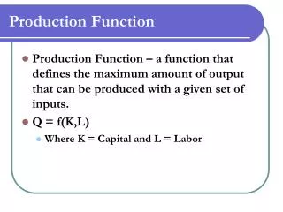
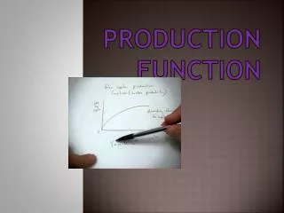
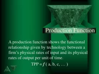
Production Function • a production function is a function that specifies the output of a firm, an industry, or an entire economy for all combinations of inputs. • A production function can be defined as the specification of the minimum input requirements needed to produce designated quantities of output, given available technology.
Production function as an equation • In a general mathematical form, a production function can be expressed as: • Q = f(X1,X2,X3,...,Xn) • where: • Q = quantity of output • X1,X2,X3,...,Xn = factor inputs (such as capital, labour, land or raw materials). This general form does not encompass joint production, that is a production process, which has multiple co-products or outputs.
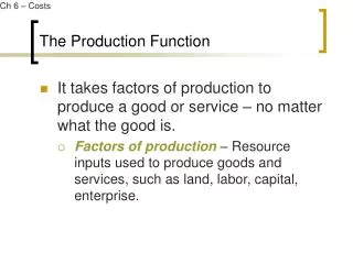
Production functions Production functions demonstrate the relationship between the amounts of inputs and the quantities of output that a firm produces.
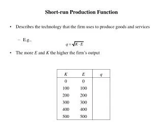
Long Run vs. Short Run • In the long run, the quantities of all inputs may be changed. All inputs are variable. The long run is sometimes referred to as the planning horizon. • In the short run, at least one input is fixed. Capital is usually assumed to be fixed in the short run. Production takes place in the short run.
Product- Total, Marginal, and Average Total product refers to the total output produced. Marginal Product When labor is combined with a fixed amount of capital, the additional output gained from additional units of labor is termed the marginal product of labor. Average product is the quantity of output per worker.
Product- Total, Marginal, and Average • Average product will… • Increase when marginal product is greater than the initial average product. • Decrease when marginal product is less than average product. • Remain constant when marginal product is equal to average product.
Product- Total, Marginal, and Average Marginal Product = ∆output/ to ∆labor Average Product = Total Product/Total Labor
Production function with two variable input (Short Run)
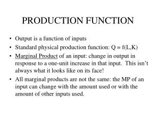
Shortrun Analysis of Prduction function Law of Variable Proportions • Law of Variable Proportions is also known as the Law of Diminishing Returns. The law states: When increasing amounts of one factor of production are employed in production along with a fixed amount of some other production factor, after some point, the resulting increases in output of product become smaller and smaller. • (That is, first the marginal returns to successive small increases in the variable factor of production turn down and then eventually the overall average returns per unit of the variable input start decreasing.)
Law of Diminishing Returns Marginal product is subject to thelaw of diminishing returnswhich states that, when additional units of labor or any other variable input are added to a fixed input, the marginal product of the variable input must eventually decrease.
Law of Diminishing Returns Negative marginal product Decreasing marginal product Increasing marginal product Quantity of output Labor
Marginal and Average Product The table shows the calculation of marginal product, which is shown in the graph. When marginal product is greater than average product, average product will increase. When marginal product is less than average product, average product will decrease. The table also shows the calculation of average product, which is plotted in the graph.
Negative marginal product Decreasing marginal product Increasing marginal product Quantity of output Qty of Labor
In which stage the rational decision is possible Assume a1,a2,a3 are units of variable factor B1,b2,b3 are units of fixed factor • Stage I is characterized by increasing AP, so that TP must also be increasing. This means that the efficiency of the variable factor of production is increasing. Fixed factor efficiency is also increasing
In which stage the rational decision is possible • The stage II is characterized by decreasing AP and a decreasing MP , but with MP not negative. Thus efficiency of the variable factor is falling, while the efficiency of b, the fixed factor, is increasing since the TP with b1 continues to increase. • Finally, the stage III is characterized by falling AP and MP, and further by negative MP. Thus the efficiency of both the fixed and variable factor is decreasing
In which stage the rational decision is possible Rational Decision: Stage II becomes the relevant and important stage of production. Production efficiency possible from the factor for which he is paying will not take place in either of the other two stages. Thus a rational producer will operate in Stage II . Suppose b is a free resource; ie it commanded no price producer would want to achieve the greatest efficiency for the factor for which he is paying, ie from factor a. Thus, he would want to produce where AP is maximum ie between Stage I & II
In which stage the rational decision is possible If a is the free resource, then he would want to employ b to its most efficient point; this is the boundary between stage II and stage III. Obviously , if both resources commanded a price, he would produce somewhere in Stage II. At what place in this production takes place would depend upon the relative prices of a and b.
ISOQUANT • ISOQUANT IS A CURVE REPRESENTING THE VARIOUS COMBINATION OF TWO INPUTS THAT PRODUCE THE SAME AMOUNT OF OUTPUT. • Iso product curve/ equal product curve / Production indifference curve
Iso quant - application • The iso quant deals with the cost-minimization problem of producers. • Isoquants are typically drawn on capital-labor graphs, showing the trade off between capital and labor in the production function, and the decreasing marginal returns of both inputs.
Iso quant - application • Adding one input while holding the other constant eventually leads to decreasing marginal output, and this is reflected in the shape of the isoquant. • An isoquant shows that the firm in question has the ability to substitute between the two different inputs at will in order to produce the same level of output.
6 A B 5 Unit Of Capital 4 C D IQ 3 4 5 8 6 Unit of labour
Properties of IQ curve • An isoquant is downward sloping to the right • Higher isoquant represents larger output • No two isoquants intersect or touch each other • Isoquants are convex to the origin • Isoquants need not be parallel to eachother • No isoquant can touch either axis
Marginal rate of technical substitution • In economics, the marginal rate of technical substitution (MRTS) or the Technical Rate of Substitution (TRS) is the amount by which the quantity of one input has to be reduced when one extra unit of another input is used, so that output remains constant ( y=y).
Marginal rate of technical substitution • Along an isoquant, the MRTS shows the rate at which one input (e.g. capital or labor) may be substituted for another, while maintaining the same level of output. The MRTS can also been seen as the slope of an Isoquant at the point in question. Since the Isoquant is generally downward sloping and marginal products are generally positive, the MRTS is generally negative.
MRTS LC = ∆C / ∆L. This can be understood with isoquant schedule MRTS
Types of isoquant • Linear isoquant- perfect substitutability. • Input output isoquant – Zero substitutability. • Kinked isoquant - limited substitutability. • Smooth convex isoquant – continuous substitutability only over a certain range .
perfect substitutability. Isoquant Units of capital Units of labour
Inputs that are perfect complements. Zero Substitutability
Limited substitutability Y P1 p2 p3 p4 Labour X capital
Imperfect Substitution Unit Of Capital IQ Unit of labour
ISO QUANT MAP/ Equal Product Map • An isoquant map where Q3 > Q2 > Q1. A typical choice of inputs would be labor for input X and capital for input Y. More of input X, input Y, or both is required to move from isoquant Q1 to Q2, or from Q2 to Q3.
Economic Region of Production : The Ridge Lines P E C A o B D F
Input prices and isocost line • Iso cost line It is the line which shows the various combination of factors that will result in the same level of total cost.
Alternative factor combinations-isocost line 5 A B 4 C Capital 3 2 4 10 Labour
The Optimum combination of inputs • a) Production of given output at minimum cost • b) Production of maximum output with a given level of cost
a) Production of given output at minimum cost K2 K1 K0 K* X1 0 L0 L1 L2 L*
Expansion path • Expansion path is the locus of different points of equilibirium when the firm’s production expenditure changes, input prices remaining constant.
The Expansion Path P E Expansion path C A o B D F
Long run production function -Returns to scale All factors are variable Eg- L & K Both l&k vary in same proportion (does not leads to change in ratio or techniques of production) or In different proportion (leads to change in ratio techniques of production with change in output) The percentage change in output when all inputs vary in the proportion is known as returns to scale.