Download
1 / 14
140 likes | 273 Views
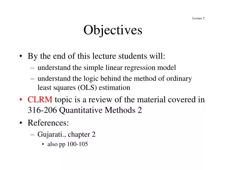
Objectives. Lecture 2. By the end of this lecture students will: understand the simple linear regression model understand the logic behind the method of ordinary least squares (OLS) estimation CLRM topic is a review of the material covered in 316-206 Quantitative Methods 2 References:

E N D
Objectives Lecture 2 • By the end of this lecture students will: • understand the simple linear regression model • understand the logic behind the method of ordinary least squares (OLS) estimation • CLRM topic is a review of the material covered in 316-206 Quantitative Methods 2 • References: • Gujarati., chapter 2 • also pp 100-105
The Model • True Model (Population Regression Function) • Yi is the ith observation of the dependent variable • Xi is the ith observation of the independent or explanatory variable • ui is the ith observation of the error or disturbance term • and are unknown parameters (coefficients) • i = 1,..., n observations
The Model • Estimated model (Sample Regression Function) • where • are the estimators of the coefficients (parameters) • are the i estimated residuals • Objective: estimate the PRF on basis of SRF
The Model • In terms of the SRF the observed Yi can be written as • in terms of the PRF Yi can be written as • Given the SRF is an approximation to the PRF can we make this approximation as close as possible?
The Model Y Yi Yi ui E(Y|Xi) E(Y|Xi) X Xi
Ordinary Least Squares (OLS) • OLS obtains the estimators and minimising the sum of squared residuals (RSS) with respect to and : • Partially differentiate RSS w.r.t. the coefficients
Ordinary Least Squares (OLS) • The first order conditions are: • (1) • (2)
Ordinary Least Squares (OLS) • Solving (1) and (2) simultaneously gives • and • where and are the sample means
Ordinary Least Squares (OLS) • Example: Melbourne house prices • Y price of house in A$’000 • X distance of house from GPO in kilometres • A=area of house in square metres • Interpret the results
Ordinary Least Squares (OLS) • What type of data is this? • Calculate the missing values of Y-hat and u-hat in the table
Ordinary Least Squares (OLS) • CHECK THE ANSWERS YOURSELVES!
Summary and conclusions • PRF vs SRF • OLS methodology • Next lecture • Gujarati p65 – 76 (Classical Assumptions) • Gujarati p107 – 112 (Normality Assumption)