Download
1 / 13
130 likes | 256 Views
Aggregate Supply. Frederick University 2014. Long Run vs. Short Run from a Macroeconomic Perspective. Long run period in macroeconomics the changes in the prices of production factors and in the prices of final goods and services are entirely synchronized Short run in macroeconomics

E N D
Aggregate Supply Frederick University 2014
Long Run vs. Short Run from a Macroeconomic Perspective Long run period in macroeconomics • the changes in the prices of production factors and in the prices of final goods and services are entirely synchronized Short run in macroeconomics • the changes in the prices are notsynchronized
Aggregate Supply (AS) AS – the willingness and ability of firms to produce GDP at every price level, ceteris paribus
Deriving AS - short run PPFandPotential GDP • The economy is in pointU – high unemployment And excess capacity – low AD. The firms would Increase production at the current price level (they do not need to be motivated by a price increase) Physical PPF А W 2. The economy moves to pointV – due to the law of diminishing returns МС start rising. The firms would increase production if only their buyers are willing to compensate them for the cost increase. Since АС grow more slowly than МС (short run and fixed cost), the increase in production is faster than the increase in the price level, i.е. production will increase faster than the price level until it gets to pointW Institutional PPF V U В
Deriving AS - short run Potential GDP and AS AS Physical PPF CPI Z Institutional PPF W Z W V V U U Real GDP At point Wthe economy operates at full capacity, MRPL = MCL; any further increase in production will be accompanied by a faster increase in cost. The firms would increase production if only their buyers are willing to compensate them for the cost increase – the price level will rise faster than output – the economy will move from point W to point Z
ASAnalysis – short run AS segments in the short run: • Horizontal Е = ∞ - from U to V – the firms are willing to increase production at the current price level; the economy operates at excess capacity • Shallow Е > fromV to W – output rises faster than the price level • E = 1 – point W – the economy operates at full capacity on the Institutional PPF and produces potential GDP; the rate of unemployment is equal to the natural rate • SteepE < 1 – from W to Z – the economy operates at overcapacity – prices increase faster than output • Vertical Е = 0 – from Z – firms cannot increase output whatever the price level is. The economic activity is on its physical PPF
ASanalysis – short run • Slope of theAScurve in the short run – determined by the law of diminishing returns and the price adjustment to cost increase • Short run – the macroeconomic perspective – the period, during which, the changes in the prices final goods and services and in the prices of production factors are not synchronized.
Factors, determining AS - short run Cost of production: • Labor cost – depends on education, traditions (attitude to work and leisure), labor supply, competitiveness of the market structure, expectations, productivity • Capital cost – depends on the savings and investment structure, raw material supplies, technological changes, competitiveness of capital markets • Government policies – regulations, taxation, social programs • Foreign sector – barriers to international trade, structure of the balance of payments
Macroeconomic Equilibrium – short run CPI AS AD1 AD Y1 – Y* =inflationary gap Y* - Y2 = recessionary gap AD2 Real GDP Y* Y1 Y2
Potential GDP andAS– long run • Potential GDP(Y*) – the level of output, which could be achieved given the physical and institutional constraints of the economic activity (full employment GDP) • Full employment – the employment level, determined by the potential output • Natural rate of unemployment (U*) – the rate of unemployment at the potential GDP level.
Potential GDP andAS– long run CPI LRAS Long run – the increase in the overall price level and in the prices of production Factors are entirely synchronized. In the long run, the increase in the prices of final goods and services does not motivate the firms to increase output, since their cost would increase at the same rate. Real GDP Y*
Potential GDP andAS– long run Factors, determining ASin the long run: • Labor resources – quantity and quality, productivity, education, traditions, motivation, demographic factors • Capital resources – quantity and quality, rate of capital accumulation • Technological changes • Institutional changes
Macroeconomic equilibrium in the long run CPI AS AD Real GDP