Download
1 / 16
190 likes | 381 Views
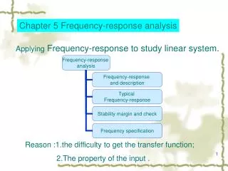
Frequency Response Analysis. Chapter 8. Outline. Segway from earlier work Fundamental Theorem of Linear Systems Graphical representations of TFs Bode Diagrams (Section 8.2) Bode Diagrams with Matlab (Section 8.3)

E N D
Frequency Response Analysis Chapter 8
Outline • Segway from earlier work • Fundamental Theorem of Linear Systems • Graphical representations of TFs • Bode Diagrams (Section 8.2) • Bode Diagrams with Matlab (Section 8.3) • Phase and Gain margins; Resonant Peak Magnitude and Resonant Frequency; Correlation between step transient response and Frequency Response in standard 2nd order system (some of Section 8.9) See FE Reference • Ungraded HW. A problems: 15, 16 (def of bandwidth), 19 (need def of miniphase) • Graded HW. B problems: 1, 2, 4 (check with Sysquake), 6, 26, 27, 29
Segway from earlier work We have solved several forms of a problem in the past. We will re-solve a form of this problem now. The solution process reviews several issues that allow us to solve the central result that forms the foundation of frequency analysis. Consider computing the acceleration that a spring-mass-damper system experiences when it is released from rest.
Hanging Spring Mass Damper Prototype form Prototype parameters and problem parameters: Ink/chalk/lead/space saving names:
Transfer Functions Relating position to input Relating acceleration to input Acceleration due to a step input Inverse Laplace transforming
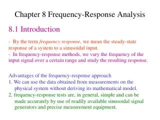
Fundamental Theorem of Linear Systems Summarizes the steady state response of a stable linear time invariant system to a sinusoidal input. Sinusoidal inputs are common in nature, are easy to obtain in the lab. Consider a stable system with transfer function G(s) and input
Compare input function to steady-state output. Draw conclusions. Magnitude and phase of G(s) are important.
Graphical Representation of TFs Bode plots. Nyquist plots. Polar plot: parameter
Phase and Gain margins See FE manual. Compare with 562 and 563.
Resonant Peak Magnitude and Resonant Frequency Consider 2nd order prototype system. Put TF in Magnitude/phase (I.e. polar) form. Find frequency of maximum magnitude (resonant frequency). Find corresponding Maximum magnitude (resonant peak magnitude). A large resonant peak magnitude indicats the presence of a pair of dominant closed loop poles with small damping ratio. (BAD) A smaller resonant peak magnitude indicates a well damped closed loop system. (GOOD). Resonant frequency is real only for damping ratio less than .707. No closed loop resonance for damping ratio greater than .707.
Correlation between step transient response and Frequency Response in standard 2nd order system Consider unity gain negative feedback system with Phase margin is See pg. 570. Cross over frequency is