Numerical Measures of Central Tendency

1. Numerical Measures of Central Tendency

2. Central Tendency Measures of central tendency are used to display the idea of centralness for a data set. Most common measures Mean Median Mode Midpoint Midrange

3. Median MD Medianis the middle value in a distribution when all values are rank ordered. It is not influenced by extreme values. It simply divided the upper half of the distribution from the lower half.

4. Properties of Median • Median is used to find the center of the data set • Can use the median to determine if values fall in the upper or lower portion of the data set • Median is not really affected by outliers that are extremely high or low

5. Median Rule of Thumb • Which value is the Median? • The rule of thumb for calculating the median is this: The median is observation (n+1)/2 • Order the observations • Calculate (n+1)/2 • Count the data values (x) until you find that observation • If you get a .5, the median is the average of those two values • Ex • n = 8: Median value is (8+1)/2 = 4.5 • The Median is the average of the 4th and 5th observations • n = 7: Median value is (7+1)/2 = 4 • The Median is the 4th observation

6. Median Examples • Data set is: 3, 5, 7, 7, 8 • n = 5 • Median value is 5+1/2 = 3rd value • MD = 7 • Data set is: 3, 5, 7, 7, 8, 10, 12, 14 • n = 8 • Median value is 8+1/2 = 4.5th value • 7 + 8 = 15/2 = 7.5 • MD = 7.5

7. Median for Grouped Data • You will do the same calculations for the continuous data • Calculate (n+1)/2 • However, the observations are already ordered for us – by the frequencies of the classes • We find the observation number by looking at the frequency of the classes

8. Grouped Data Set • To Calculate the median, we find (n+1)/2 • n = 8 • (8+1)/2 = 4.5 • It is the average of the 4th & 5th observations • Use Class Midpoints for observation values • 4th values is 2 • 5th value is 7 • Average is (7+2)/2 = 4.5 • MD = 4.5 Observations 1, 2, 3, & 4 Observations 5 & 6 Observation 7 Observation 8

9. Mode • The mode is the most frequent observation. The distribution may have several modes or no modes. • Only measure of central tendency that can be used for categorical data • Types of Modes • Unimodal –one mode • Bimodal –two modes • two values that occur with identical highest frequency • Multimodal –more than two modes • No mode –every observation occurs only once

10. Mode 3 5 1 4 2 9 6 10 Rank Ordered: 1 2 3 4 5 6 9 10

11. Mode 3 5 1 4 2 9 6 10 5 3 4 3 9 3 6 1 Rank Ordered: 1 1 2 3 3 3 3 4 4 5 5 6 6 9 9 10

12. Mode 6 10 5 3 4 3 9 3 6 1 6 Rank Ordered: 1 3 3 3 4 5 6 6 6 9 10

13. Grouped Data • Instead of a mode, we have a modal class • Determine the class with the highest frequency • The modal class is 0 – 4

14. Midrange • The midrange, MR, is a more rough estimate of the middle of the data set • Found by taking the average of the highest and the lowest values • Affected by outliers

15. Midrange Examples • Data set is: 3, 5, 7, 7, 8 • Midrange value is (8 + 3)/2 = 5.5 • MR = 5.5 • Data set is: 3, 5, 7, 7, 8, 10, 12, 14 • Midrange value is (14 + 3)/2 = 8.5 • MR = 8.5

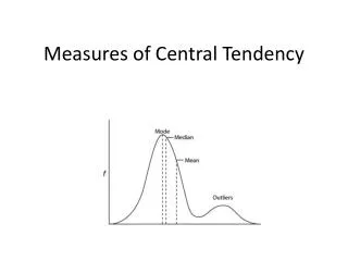
16. Distribution When the mean, median, and mode are all at the same point, the center of the distribution, the data is considered to be symmetrically or normally distributed.

17. Distribution When data is skewed, values have “bunched” up at one end or the other. With skewed data, the mean, median, and mode are usually all different values (spread apart). The distribution of the data can be positively or negativelyskewed.

18. Distribution Positively skewed distribution (Mode < Median < Mean) A distribution in which the majority of the data values fall to the left of (below) the mean. The tail of the data trails to the upper end of the values

19. Distribution Negatively skewed distribution (Mean < Median < Mode) A distribution in which the majority of the data values fall to the right of (above) the mean. The tail of the data trails to the lower values of the data