Download
1 / 64
650 likes | 949 Views
Chaps. 7 & 8: Sequence Alignment. Pairwise Alignment Given two sequences, how similar are they ? Dynamic Programming Multi-sequence Alignment. Sequence Alignment. Example Mitochondrial cytochrome b From NCBI protein web page, search for cytb and Loxodonta africana (African elephant)

E N D
Chaps. 7 & 8: Sequence Alignment • Pairwise Alignment • Given two sequences, how similar are they ? • Dynamic Programming • Multi-sequence Alignment
Sequence Alignment • Example • Mitochondrial cytochrome b • From NCBI protein web page, search for cytb and • Loxodonta africana (African elephant) • Elephas maximus (Indian elephant) • Mammuthus primigenius (Siberian wooly Mammoth) • Which modern elephant is closer to a mammoth ? • Use clustalW to do the alignment
>0012AAX12542.1| cytochrome b [Elephas maximus] MTHTRKSHPLFKIINKSFIDLPTPSNISTWWNFGSLLGACLITQILTGLFLAMHYTPDTMTAFSSMSHIC RDVNYGWIIRQLHSNGASIFFLCLYTHIGRNIYYGSYLYSETWNTGIMLLLITMATAFMGYVLPWGQMSF WGATVITNLFSAIPYIGTNLVEWIWGGFSVDKATLNRFFAFHFILPFTMVALAGVHLTFLHETGSNNPLG LTSDSDKIPFHPYYTIKDFLGLLILILLLLLLALLSPDMLGDPDNYMPADPLNTPLHIKPEWYFLFAYAI LRSVPNKLGGVLALLLSILILGLMPLLHTSKHRSMMLRPLSQVLFWALTMDLLMLTWIGSQPVEYPYIAI GQMASILYFSIILAFLPIAGMIENYLIK >gi|56578537|gb|AAW01445.1| cytochrome b [Loxodonta africana] MTHIRKSYPLLKIINKSFIDLPTPSNISAWWNFGSLLGACLITQILTGLFLAMHYTPDTMTAFSSMSHIC RDVNYGWIIRQLHSNGASIFFLCLYTHIGRNIYYGSYLYSETWNTGIMLLLITMATAFMGYVLPWGQMSF WGATVITNLFSAIPYIGTNLVEWIWGGFSVDKATLNRFFALHFILPFTMTALAGVHLTFLHETGSNNPLG LTSDSDKIPFHPYYTIKDFLGLLILILLLLLLALLSPDMLGDPDNYMPADPLNTPLHIKPEWYFLFAYAI LRSVPNKLGGVLALFLSILILGLMPLLHTSKYRSMMLRPLSQVLFWTLTMDLLMLTWIGSQPVEYPYTII GQMASILYFSIILAFLPIAGMIENYLIK >gi|2924604|dbj|BAA25008.1| cytochrome b [Mammuthus primigenius] MTHIRKSHPLLKILNKSFIDLPTPSNISTWWNFGSLLGACLITQILTGLFLAMHYTPDTMTAFSSMSHIC RDVNYGWIIRQLHSNGASIFFLCLYTHIGRNIYYGSYLYSETWNTGIMLLLITMATAFMGYVLPWGQMSF WGATVITNLFSAIPYIGTDLVEWIWGGFSVDKATLNRFFALHFILPFTMIALAGVHLTFLHETGSNNPLG LTSDSDKIPFHPYYTIKDFLGLLILILFLLLLALLSPDMLGDPDNYMPADPLNTPLHIKPEWYFLFAYAI LRSVPNKLGGVLALLLSILILGIMPLLHTSKHRSMMLRPLSQVLFWTLATDLLMLTWIGSQPVEYPYIII GQMASILYFSIILAFLPIAGMIENYLIK
Pairwise sequence alignment is the most fundamental operation of bioinformatics It is used to decide if two proteins (or genes) are related structurally or functionally It is used to identify domains or motifs that are shared between proteins It is the basis of BLAST searching (next) It is used in the analysis of genomes
Direct Alignment • Given two sequences • +1 if letters in the same positions match • -1, otherwise • Extremely simple, but what if there is a gap? • Gap when a base is inserted or deleted • Maybe only in biological data • Maybe more significant mutation – give more negative score as a penalty RNDKPFSTARN RNQKPKWWTA + + - + +- - - - - -
Visual Alignment -- Dotplot • A seq. in x axis and the other in y axis • Dot on a crosspoint if identical in both sequences • view
Special Dotplot Periodic Palindrome
Similarity and Homology • Similarity • Observation or measurement of resemblance, independent of the source of the resemblance • Can be observed now but involves no historical hypothesis • Homology • Specifies that sequences and the organisms descended from a common ancestor • Implies that similarities are shared ancestral characteristics • Cannot make the assertion of homology from historical evidence, and thus is an inference from observations of similarity
Homology • Similarity attributed to descent from a common ancestor • Two types of homology • Orthologs • Homologous sequences in different species that arose from a common ancestral gene during speciation; may or may not be responsible for a similar function. • Paralogs • Homologous sequences within a single species that arose by gene duplication.
Orthologs: members of a gene (protein) family in various organisms. This tree shows globin orthologs.
Paralogs: members of a gene (protein) family within a species. This tree shows human globin paralogs.
Sequence Alignment g c t g a a c g c t a t a a t c g c t g - a a - c g - c t a t a a t c - g c t g - a a - c - g - - c t - a t a a t c • Direct alignment • An alignment with gaps • What is the criteria for a good alignment ? • Use score to check for optimality • May not produce a unique optimal alignment
Calculation of an alignment score Source: http://www.ncbi.nlm.nih.gov/Education/BLASTinfo/Alignment_Scores2.html
General approach to pairwise alignment Given two sequences Select an algorithm that generates a score Allow gaps (insertions, deletions) Score reflects degree of similarity Alignments can be global or local Estimate probability that the alignment occurred by chance
Pairwise alignment: protein sequencescan be more informative than DNA • protein is more informative (20 vs 4 characters); many amino acids share related biophysical properties • codons are degenerate: changes in the third position often do not alter the amino acid that is specified • protein sequences offer a longer “look-back” time • DNA sequences can be translated into protein, and then used in pairwise alignments • Many times, DNA alignments are appropriate when • to confirm the identity of a cDNA • to study noncoding regions of DNA • to study DNA polymorphisms • example: Neanderthal vs modern human DNA
Scoring Matrix • Dotplot • Incredibly useful in identifying biological significance and interesting regions • Do not privde a measure of statistical similarity • A numerical method • Not just provide position-by-position overlap • But provide the nature and characteristics of residues being aligned • Scoring matrices • Empirical weighting schemes
Scoring Matrix • Three biological factors in constructing a scoring matrix • Conservation • Account for conservation between proteins, but provide a way to assess conservation substitutions • Score represents what residues are capable of substitution for other residues while not adversely affecting the function of the native protein (determined by charge, size, hydrophobicity, etc.) • Frequency • Reflect how often residues occur among proteins • Rare residues are given more weight • Evolution • By design, implicitly represent evolutionary patterns • Review • http://books.google.com/books?hl=en&lr=&id=9p3E2sS1aJUC&oi=fnd&pg=PA73&ots=eJ0lzjEg_b&sig=Fl2kBl5QBq7VIoy-eDgDqXhaZ14#v=onepage&q&f=false
Scoring Matrix • Log-Odds Score • qij : prob. of how often i and j are seen aligned • pi: prob. of observing AA I among all proteins • sij = log(qij/ pipj) • score • Represent the ratio of observed versus random frequency of substitutign i by j • Positive score – two residues are replaced more often than by chance • Negative – less likely to substitute than by chance
BLOSUM62 • Most popular • diagonal • Score for exact match • W-W: score 11: because alignment of W between two sequences is rare • Off-diagonal • W (tryptophan) – Y (tyrosine): score 2 • Positive score – occur more often than by chance, but replacement is not as good as if W is preserved (2 < 11) or if Y is preserved (2 < 7) • W – V (Valine): score -3
Scoring Matrix • 1978 – Dayhoff, Schwartz, Orcutt • From aligned sequences of 71 families of closely related proteins (sharing more than 85% of sequences), tabulated 1572 substitutions • Substitutions are considered “accepted” mutations in phylogenetic tree • AA change accepted by natural selection occurs when • A gene undergoes a DNA mutation to translate to a different AA and does not significantly alter the gene function • The entire species adopts the change as a predominant form of the protein • Frequencies can represent expected mutation over short evolutionary distances • Called PAM (Point Accepted Mutation) • PAM unit corresponds to one AA change per 100 residues (1% divergence)
PAM matrix • assumptions • Most important assumption – each AA replacement is independent of previous mutations at the same position • Matrix can be extrapolated into predicted substitution fequencies at longer evolutionary distances • PAM1 multiplied by itself 100 times can represent what one would expect if there were 100 AA changes per 100 residues – PAM100 • All sites are equally mutable independent of neighboring residues • No consideration of conserved blocks or motifs • Forces responsible for sequence evolution over shorter time span are identical to those for longer time spans • 1992 – Jones, Taylor, Thornton (JTT) • 59,190 substitutions in all sequences in Swiss-Prot
Protein Substitution Rates Protein Substitution Rates • Example • Six letters: I, K, L, Q, T, V • Seven sequences • Form an evolutionary tree A: T L K K V Q K T B: T L K K V Q K T C: T L K K I Q K Q D: IIT K L Q K Q E: T I T K L Q K Q F: T L T K I Q K Q G: T L T Q I Q K Q
Protein Substitution Rates • Determine AAij • Count AA j being substituted by i I K L Q T V I - - 2 - 1 1 K - - - 1 1 - L 2 - - - - - Q - 1 - - 1 - T 1 1 - 1 - - V 1 - - - - -
Dayhoff counting • Most freq. subs.: Glu to Asp (both acidic)
Sub. Frequency to Score Matrix • AA mutation prob. • Mij : Prob. of original AA j mutating to AA i in one PAM distance • PAM distance: unit of evolutionary divergence in which 1% of AA's have changed between two protein sequences • Mij = Aij /Ni (Ni count of amino acid i) -- normalized by the prob. of AA i occurring • Pij(t) : Prob. that a site has AA i at time t when it had j at time 0 • Pij(dt) = Mij
Mutation Prob. Matrix • Each entry is scaled by 105 • Two most freq. substitutions are highlighted
Sub. Frequency to Score Matrix • 2. Mutation Prob. Matrix to Log-Odds Scoring • qij : Prob. of aligning j to i • pi: prob. of observing AA i by chance • sij = 10*log(qij/ pi) • e.g., sED = 10*log(0.00398/0.062) • Can add log-odd scores
PAM1 matrix • Mutation Prob. Matrix has Pij(t) • PAM1 matrix for related proteins with 1% mutation • = 99% identical between two sequences • For distantly related proteins, other PAM matrices are used by successively multiplying PAM1 • PAM250 is used for BLAST PAM 0 30 80 110 200 250 % identity 100 75 60 50 25 20
Pairwise Alignment vs. PAM Distance • Two sequences 100 AAs • After 80 PAM distances (80 mutations), 50 AAs are different • After 150 hits, 20 AAs remain the same
PAM matrices • Closely related: Human vs. Chimpanzee (100% AA identical) • Distantly related: HBA vs. HBB (43% AA identical)
BLOSUM • S.Henikoff and J.G. Henikoff • Devised to perform best in identifying distant relationships • Based on BLOCKS database of aligned protein sequences • BLOcks Substitution Matrix • (# of observed pairs of AA at any position)/(# of pairs expected from the overall AA frequencies) is computed from regions of closely related proteins alignable without gaps • To avoid overweighting closely related sequences, groups of proteins with sequence identities higher than a threshold are replaced by either a single representative or a weighted average
BLOSUM 62 • BLOSUM Threshold set at 62 • Protein sequences sharing less than 62% identity • Default BLAST
Other Scores • Gap penalty • Gap initiation and extension • Clustal-W recommends use of identity matrix • For DNA sequences • 1 for a match, 0 for a mismatch, gap penalty of 10 for initiation and 0.1 for extension per residue • For AA sequences • BLOSUM62 matrix for substitution, gap penalty of 11 for initiation and 1 for extension per residue a a a g a a a a a a – a a a a a a g g g a a a a a a - - - a a a
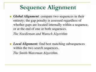
Pairwise Alignment: Global and Local • Given a scoring scheme, find alignments maximizing the score • Global • Entire sequence of protein or DNA sequence • Needleman and Wunsch (dynamic programming) • Local • Focus on regions of greatest similarity • Smith and Waterman • In general, preferable to Global Alignment • Because only portions of proteins align
Dynamic Programming • Guaranteed to yield an optimal global alignment • Drawback – many alignments may give the same optimal score and none of them may correspond to biologically correct alignment • W.Fitch and T.Smith found 17 alignments of alpha- and beta-chains of chicken haemoglobin, one of which is correct based on structures • Drawback – complexity O(nm) for sequences of length n and m
Dynamic Programming • Rock removal game • Two piles of rocks, each with 10 rocks • A and B alternatively remove one rock from a single pile or one rock each from both piles • Player who remove the last rock(s) wins the game • Use reduction strategy starting with smaller problems • Consider 2+2 problem • A removes one rock each, B removes one rock each • A removes one rock, B takes one rock from the same pile • B wins • 3+3 problem ?
Rock Removal with 10+10 • ↑ A takes one from pile X • ← A takes one from pile Y • A takes one from each pile • * A will lose
Manhattan Tourist Problem • Visit as many tourist sites in a Manhattan grid • Move to the east or south only • Start at upper left corner • End at # 15, lower right corner
Problem Statement • Given a weighted grid G with two vertices (nodes) for a source and a sink • Find the longest path in a weighted grid • Weight: # of attraction sites on an edge (link) • Each vertex (node) can be identified by (i,j) • Source at (0,0) • Sink at (n, m) 3 2 4 1 0 2 4 3 2 4 4 6 5 2 0 7 3 4 4 5 2 3 3 0
Solution (0,0) • Define si,j: the longest path from source to vertex (i,j) (0≤i<n, 0 ≤j<m) • Solve for smaller problems first • Solving for s0,j and si,0 is easy 3 2 4 0 3 5 9 1 0 2 4 3 2 4 1 4 6 5 2 0 7 3 5 4 4 5 2 3 3 0 9
Solution (2) (0,0) (0,1) 3 2 4 • Iteratively solve for neighboring nodes • si,1 • si,2, etc. 0 3 5 9 1 0 2 4 (1,0) 3 2 4 1 4 4 6 5 2 (2,0) 0 7 3 5 10 4 4 5 2 (3,0) 3 3 0 9 14 • si,j= max[si-1,j + weight on edge between (i-1,j) and (i,j), • si,j-1 + weight on edge between (i,j-1) and (i,j)]
Algorithm • Algorithm • Given Weast(i,j) and Wsouth(i,j), • s0,0 = 0 • for i =1 to n • si,0 = si-1,0 + Wsouth(i,0) • for j =1 to n • s0,j = s0,j-1 + Weast(0,j) • for i =1 to n • for j = 1 to m • si,j = max[si-1,j + Wsouth(i,j), • si,j-1 + Weast(i,j)] • return sn,m
General Graph Problem • Not regular with two inputs (indegree) and two outputs (outdegree) at a node
Directed Acyclic Graph • DAG: Directed Acyclic Graph • G = (V, E) • Longest Path Problem • sv = max(su + weight from u to v) over all u which are Predecessor(v) • Predecessor relationship has to be established ahead of the time u1 5 7 3 u2 v 5 u3