Download
1 / 6
60 likes | 80 Views
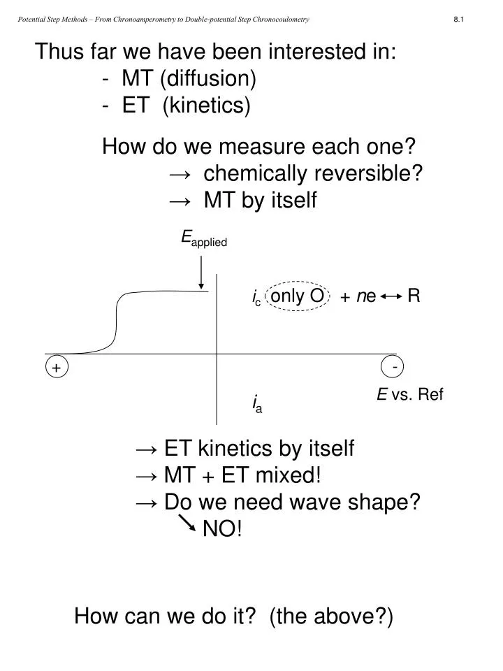
Potential Step Methods – From Chronoamperometry to Double-potential Step Chronocoulometry. 8.1. Thus far we have been interested in: - MT (diffusion) - ET (kinetics). How do we measure each one? → chemically reversible? → MT by itself. E applied. i c only O + n e R. +.

E N D
Potential Step Methods – From Chronoamperometry to Double-potential Step Chronocoulometry 8.1 Thus far we have been interested in: - MT (diffusion) - ET (kinetics) How do we measure each one? → chemically reversible? → MT by itself Eapplied iconly O + ne R + - E vs. Ref ia • ET kinetics by itself • MT + ET mixed! • Do we need wave shape? NO! How can we do it? (the above?)
Response i(t) ? time (sec) Potential Step Methods – From Chronoamperometry to Double-potential Step Chronocoulometry 8.2 Consider an E-step experiment in unstirred soln: Excitation Efinal Eapplied Einitial time (sec) t = 0 The response is affected by: - Efinal - k0 - Do - Co* Keeping Do and Co* out of the picture, we need To worry about Efinal and k0. Let’s assume two cases (for the moment): Case I: k0 is fast (rev. ET) Case II:k0 is slow (irrev. ET) Looking at Case I, we can be at various potentials, Eapplied. Let us choose two situations: situation A: Eapp > EMT (but not too +) situation B: Eapp≤EMT
Potential Step Methods – From Chronoamperometry to Double-potential Step Chronocoulometry 8.3 Case I A: If stirred and scan E: ic EF Ei -E vs.Ref Ei EF ia time (sec) t = 0 MT limited, even if no stirring. Thus, but rather MT. Must solve FSL with necessary boundary and initial conditions: Potential Step Boundary Controls (Describes E step conditions) at t > 0 Semi-Infinite Diffusion Boundary Conditions (No at sufficient x) at t > 0 (Before Eapp, the soln is homogenous) at t = 0 Initial Conditions
1.0 0 0.4 0.8 1.2 1.6 2.0 2.4 2.8 x, cm x 103 Potential Step Methods – From Chronoamperometry to Double-potential Step Chronocoulometry 8.4 We now can do the math (see Appendix A): “l“ Get: Recall: and and Do this for: DO = 10-5 cm2 s-1 Basically: 0.001s 0.01s 0.1s 1s So, the current decays with time.
Potential Step Methods – From Chronoamperometry to Double-potential Step Chronocoulometry 8.5 Recall FFL: Sometimes we call the Cottrell Current the Diffusion Current, id(t) Substituting Cottrell Equation Characteristics of Cottrell Equation i vs. t-1/2 will be linear for diff. controlled O + ne R reaction and no “pre-kinetics” of O: +ne-
Potential Step Methods – From Chronoamperometry to Double-potential Step Chronocoulometry 8.6 Cottrell Limitations with which to be concerned: • Double Layer concerns/Rs concerns- • At early t we have bothif and iDL flowing. • Thus, imeas > if DL imeas ideal Convection! o o t-1/2 (sec-1/2) • Convection concerns (long t)- • imeas is larger than expected. • Instrument Concerns- • Potentiostat current meas. limits • (voltage compliance) • Recording Device (op ramps)