Download
1 / 16
160 likes | 334 Views
Impact of rainfall and model resolution on sewer hydrodynamics G . Bruni a , J.A.E. ten Veldhuis a , F.H.L.R. Clemens a , b a Water management Department, Faculty of Civil Engineering and Geosciences, Delft University of Technology, Stevinweg 1, 2628CN, Delft, NL

E N D
Impact of rainfall and model resolution on sewer hydrodynamics G. Brunia, J.A.E. ten Veldhuisa, F.H.L.R. Clemensa, b a Water management Department, Faculty of Civil Engineering and Geosciences, Delft University of Technology, Stevinweg 1, 2628CN, Delft, NL b Deltares, P.O. Box 177, 2600 MD Delft, The Netherlands 7th International Conference on Sewer Processes & Networks Wed 28 - Fri 30 August 2013 The Edge Conference Centre, Sheffield
Problem statement ? IMPROVEMENT OF THE DETAIL OF SEWER MODELS X-BAND DUAL POLARIMETRIC RADARS TO INCREASE THE RESOLUTION AND ACCURACY IMPROVEMENT OF RAINFALL ESTIMATE ACCURACY ENHANCEMENT OF THE USE OF RADAR RAINFALL DETAILED LAND USE INFORMATION ACCURATE INFORMATION OF SEWER CHARACTERISTICS AND PROCESSES
Casestudy Eindoven area: RioolZuid -> “Southern sewer system” North Sea The Netherlands Germany Belgium • it serves 9 municipalities (~3’000 to ~43’000 inhabitants) • 18.6 km long free-flow conduit • Sewer system detail: from~ 500 nodes to 3’800 nodes .
Dataset- Rainfall Ground measurements: 2 rain gauges Bergeijkand Vessem C-band radar data, KNMI
Dataset- model specification Model lumping • Software package: Infoworks CS • Runoff estimation model: Fixed RC (impervious areas) and Horton for infiltration losses (pervious areas) • Runoff concentration: single linear resevoir (Desbordes) • Sewer flow routing: dynamic wave approximation of the Saint-Venant equations
Methodology Simulated scenarios 2. RG-D 4. RG-L 3. RAD-L 1. RAD-D 1. RAD-D: distributed sewer model with radar rainfall in input 2. RG-D: distributed sewer model with rain gauge rainfall in input 3. RAD-L:lumped sewer model with radar rainfall in input 4. RG-L: lumped sewer model with rain gauge rainfall in input
Rainfall selection- Event 1 Storm evolution at Bergeijk and Vessem rain gauges vs overlapping radar pixels Radar storm accumulation and maximum intensity
Rainfall selection- Event 2, 3 and 4 Event 2 Event 3 Event 4
Results-1 Water level results at Bergeijk Event 1 Event 2 Event 3 Event 4
Results-2 Water level results at Westehoven-Event 2 Valkenswaard- Event 3
Results 3- differences along the main conduit 4 3 4 3 1 2 2 1 3 4 1 2
Conclusions • The impact of model structure on water levels is higher at locations close to rain gauges, i.e. when the rain gauge does accurately describe the storm evolution; • The effect of rainfall resolution on model results becomes significant at locations far from the ground measurements: rain gauge fails to describe rainfall structure; • The bias found in all six scenario pairs increases in the downstream direction, since the rain gauge is not representative of rainfall occurred at large distance (>4 km), and the lumping of larger catchments introduces higher error.
*J.W. Wilson and E.A.Brandes, 1975 E. Goudenhoofdt and L. Delobbe, 2009 Brandes spatial adjustment (BRA)* This spatial method was proposed by Brandes (1975). A correction factor is calculated at each rain gauge site. All the factors are then interpolated on the whole radar field. This method follows the Barnes objective analysis scheme based on a negative exponential weighting to produce the calibration field: where di is the distance between the grid point and the gauge i. The parameter k controls the degree of smoothing in the Brandes method. It is assumed constant over the whole domain. The parameter k is computed as a function of the mean density of the network, given by the number of gauges divided by the total area. A simple inverse relation has been chosen: k = (2δ)−1 The factor 2 was adjusted to get an optimal k for the full network. The optimal k was estimated by trial and error based on the verification for the year 2006. The same relation between k and is used for the reduced networks.