Download

1 / 36
400 likes | 856 Views
0VS452 + 5EN253 Lecture 8 – part I. Business cycles and intro to AD-AS model. Eva Hrom á dkov á , 12.4 2010. Overview of Lecture 8 – part I. Business cycles: Why do we need other than classical model? Puzzle of Great Depression Prices in the short vs. long run Intro to AD and AS curves

E N D
0VS452 + 5EN253 Lecture 8 – part I Business cycles and intro to AD-AS model Eva Hromádková, 12.4 2010
Overview of Lecture 8 – part I Business cycles: • Why do we need other than classical model? • Puzzle of Great Depression • Prices in the short vs. long run • Intro to AD and AS curves • Effect of shocks in AD-AS model • Stabilization policy – tools and goals
MotivationFailure of classical economy in the case of Great Depression Great Depression: • Before – period of rapid growth (GDP, stocks) • October 24, 1929 – Black Thursday • Crash of stock market –> sell-off • Fall of wealth, savings => depression of real sector • Output, consumption, investment falling • Unemployment: 1929 – 3%, 30’ – 9%, 33’ – 25%, 39’ – 17%
MotivationFailure of classical economy in the case of Great Depression Classical economy Reality • Assumption of self-regulating economy • Prices are flexible • Unemployment and excess supply will disappear as soon as prices will adjust • Deflation(30’ = -10%) • Still, high unemployment Keynes: • Economy is inherently unstable • Need for government intervention • Debate lasts until now
Business cyclesTerminology – What do we mean by inherently unstable? Recession: typically defined as a decline in real GDP for two or more consecutive quarters, accompanied with high unemployment Depression: any economic downturn where real GDP declines by more than 10 percent, longer and more severe than recession
Business cycles (fluctuations)Real world – Summary of example of USA Real GDP growth in US: • long-run growth of 3.5% • not steady – fluctuations around trend: • Great Depression • WWII – growth by 19%, all people employed • 46’-48’ – postwar depression (military production) • 80’s oil crisis
Business cycles (fluctuations)Stylized facts • No simple regular or cyclical pattern • Distributed unevenly over the components of output • Stable: consumption of non-durables and services, net export • Unstable: consumption of durables, housing, inventories • Asymmetries between rises and falls in output • Long time slightly above and short time far below the mean value
Business fluctuationsRole of macro theory • Macro theory tries to explain why we observe alternating periods of growth and contraction in short run; together with long-term trends • Main difference • Long-run: prices are flexible, respond to changes in supply or demand • Short run: many prices are “sticky” The economy behaves much differently when prices are sticky.
Business fluctuationsComparison of long-term and short-term determinants Long-term (classical economy) Short term (business cycles) • Price flexibility • Output determined by supply side ( F(K,L) ) • Change in demand only affects prices, not quantities • Say’s law: supply creates demand • Price stickiness • Output determined also by demand – affected by exogenous changes • Ex: firm – how much we are able to sell at given price
Model of AD and AS • the paradigm that most mainstream economists & policymakers use to think about economic fluctuations and policies to stabilize the economy • shows how the price level and aggregate output are determined simultaneously • shows how the economy’s behavior is different in the short run and long run
Aggregate demand • The aggregate demand curve shows the relationship between the price level and the quantity of output demanded. • For this lecture’s intro to the AD/AS model, we use a very simple theory of aggregate demand based on the Quantity Theory of Money. • In this and next lecture we develop the theory of aggregate demand in more detail.
Aggregate demandQuantity theory of money • From Lecture 3, recall the quantity equation MV = PY and the money demand function it implies: (M/P)d = kYwhere V = 1/k = velocity. • For given values of M and V, these equations imply an inverse relationship between P and Y: P = (M V) / Y
P AD Y Aggregate demandDownward-sloping curve Real balances effect: • Increase in price level causes fall in real money balances => decrease in demand
P AD2 AD1 Y Aggregate demandShift of AD curve – Ex.: increase in the money supply Increase in money supply => shift of AD curve to the right Explanation: • Can buy more at the same price P = (M V) / Y Rise in M
Aggregate supplyLong run AS curve In the long run, output is determined by factor supplies and technology • full-employmentor natural level of output, the level of output at unemployment equals its natural rate (no inflationary pressures). • does not depend on the price level, so the long run aggregate supply (LRAS) curve is vertical:
LRAS P Y Aggregate supplyLong run - graph • Long run AS curve is vertical at optimal Y • Classical assumption
LRAS P P2 In the long run, this increases the price level… AD2 AD1 Y …but leaves output the same. AD-AS modelLong-run effects of AD shift (increase in M) An increase in Mshifts the ADcurve to the right. P1
AD-AS modelLong-run - Implications In the long run – change in the money supply does not have any effect on real variable, only on the price level • Deviation only as long as price adjusts Not what we observe in reality! • Consider a long term outcome • Self-adjusting deviations • Economic growth based on the growth of real variables: capital, labor, technology • Analyze departures
Aggregate supplyShort run • In the real world, many prices are sticky in the short run. • From now on we assume that all prices are stuck at a predetermined level in the short run… • …and that firms are willing to sell as much as their customers are willing to buy at that price level. • Therefore, the short-run aggregate supply (SRAS) curve is horizontal: • (simplification – in reality, upward sloping)
P SRAS Y Aggregate supplyShort run AS curve SRAS is horizontal: • Price level fixed at a predetermined level • Firms sell as much as buyers demand
In the short run when prices are sticky,… P SRAS AD2 AD1 Y …causes output to rise. Y2 AD-AS modelLong-run effects of AD shift (increase in M) …an increase in aggregate demand… Y1
AD-AS modelShort-run - Implications In the short run – change in the AD (money supply) has full effect on real variable + no on price level Equilibrium may be undesirable – higher or lower output (and corresponding prices) than in natural level • Lower output – recessionary gap – high unemployment rate • Higher output – inflationary gap – pressure to increase prices
AS-AD modelFrom the short run to the long run Over time, prices gradually become “unstuck.” When they do, will they rise or fall? In the short-run equilibrium, if then over time, the price level will ? ? ?
LRAS P P2 SRAS AD2 AD1 Y Y2 AD-AS modelShort and Long-run effects of AD shift (increase in M) A = initial equilibrium B = new short-run equilib. after increase M C B A C = long-run equilibrium
AD-AS model Summary of basic model • Bad news – recessions are inevitable • Good news – hope for adjustment BUT!!! Reality strikes back • Money supply changes are predictable (CB), however, other shocks may shift both curves – unpredictable and even simultaneous • Adjustment takes a long time – do we need “nudge” from government?
AD-AS model 1. Introduction of shocks • Shocks: • exogenous changes in aggregate supply or demand • temporarily push the economy away from full-employment AD shocks AS shocks • Lower export demand • Lower consumer confidence • Taxation • Changing import prices • Natural disasters • changing input costs
CASE STUDY: The 1970s oil shocks • Early 1970s: OPEC coordinates a reduction in the supply of oil. • Oil prices rose 11% in 1973 68% in 1974 16% in 1975 • Such sharp oil price increases are supply shocks because they significantly impact production costs and prices. Q1: How would this situations look depicted in AD-AS framework?
LRAS P SRAS2 SRAS1 AD Y Y2 CASE STUDY: The 1970s oil shocks The oil price shock shifts SRAS up, causing output and employment to fall. B In absence of further price shocks, prices will fall over time and economy moves back toward full employment. A A
CASE STUDY: The 1970s oil shocks Predicted effects of the oil price shock: • inflation • output • unemployment …and then a gradual recovery.
CASE STUDY: The 1970s oil shocks Late 1970s: As economy was recovering, oil prices shot up again, causing another huge supply shock!!!
CASE STUDY: The 1980s oil shocks 1980s: A favorable supply shock--a significant fall in oil prices. As the model would predict, inflation and unemployment fell:
AS-AD model2. Stabilization policy • Definition: policy actions aimed at reducing the severity of short run economic fluctuations • Types: • Laissez faire – no action, economy will self-adjust to optimal position • Fiscal policy: gvt expenditures, taxation (AD side) • Fiscal multiplier • Monetary policy: money supply and interest rates • Money multiplier • Supply side policy: incentives for work, saving, investment • Trade policy: e.g. reducing trade barriers
LRAS P SRAS2 SRAS1 AD1 Y Y2 AS-AD model2. Stabilization policy – example of supply shock The adverse supply shock moves the economy to point B. B A
LRAS P SRAS2 AD2 AD1 Y Y2 AS-AD model2. Stabilization policy – example of supply shock But CB can accommodate the shock by raising agg. demand. B C A results: P is permanently higher, but Y remains at its full-employment level.
AD-AS modelStabilization policy - concerns • Which type of policy tool is optimal? • What would be the final result? Can we account for all the injections (multiplication) and leakages? • How do we account for changing expectations? • How do we trade between inflation and unemployment?