Download
1 / 22
220 likes | 371 Views
Coupling COSMO with the WAM model. Aron Roland (TUD, Darmstadt), Mathieu Dutour (IRB, Zagreb), Luigi Cavaleri (ISMAR, Venice), Luciana Bertotti (ISMAR, Venice) and Lucio Torrisi (CNMCA – Rome). Content. Motivation Physics The coupling library and it’s methodology

E N D
Coupling COSMO with the WAM model Aron Roland (TUD, Darmstadt), Mathieu Dutour (IRB, Zagreb), Luigi Cavaleri (ISMAR, Venice), Luciana Bertotti (ISMAR, Venice) and Lucio Torrisi (CNMCA – Rome). September 2, 2011 | Roland et al., EGU, 2011 | 1
September 2, 2011 | Roland et al., 2011 | 2 Content Motivation Physics The coupling library and it’s methodology Validation of the coupling library Conclusion
September 2, 2011 | Roland et al., 2011 | 3 Motivation Wind generate waves influence the atmosphere and determine the fluxes from the ocean to the atmosphere. Waves are driving currents and currents are modulating the waves. In order to have the full cycle we couple in this project the operationally used COSMO (Atmosphere) WAM (Waves) ROMS (Currents) models The leading model is here COSMO organizing the output, providing the forcing for the other two models and receiving the surface conditions from them.
September 2, 2011 | Roland et al., 2011 | 4 Motivation
September 2, 2011 | Roland et al., 2011 | 5 Some recent results of Hurricane Isabel using coupled Ocean-Wave model (SELFE-WWMII) on unstructured meshes driven by NARR (North American Regional Reanalysis) winds …
September 2, 2011 | Roland et al., 2011 | 6 Some recent results of Isabel using coupled Ocean-Wave model on unstructured meshes …
September 2, 2011 | Roland et al., 2011 | 7 Comparison of the sign. Wave height with the buoy measurements (blue no currents, black with currents)
September 2, 2011 | Roland et al., 2011 | 8 Comparison of the average period with the buoy measurements
September 2, 2011 | Roland et al., 2011 | 9 Estimation Isabell storm surge
September 2, 2011 | Roland et al., 2011 | 10 Atmospheric conditions during Xynthia courtesy to Xavier Bertin, submitted to OM
September 2, 2011 | Roland et al., 2011 | 11 Xynthia !Influence of wave induced surface drag on the sea surface elevation courtesy to Xavier Bertin, submitted to OM
September 2, 2011 | Roland et al., 2011 | 12 Physical formulations – potential for improvement when coupling COSMO + WAM • When looking at the sea surface it becomes evident that the sea surface roughness depends on the sea state. • When looking at a typical balance of energy fluxes for a growing wind sea at a constant wind speed of 20m/s (Janssen et al. 2002) • “At the same time Fig. 1 illustrates the role ocean surface waves play in the interaction of the atmosphere and the ocean, because on the one hand ocean waves receive momentum and energy from the atmosphere through wind input (controlling to some extent the drag of air flow over the oceans), while on the other hand, through wave breaking, the ocean waves transfer energy and momentum to the ocean thereby feeding the turbulent and large-scale motions of the oceans”. (Janssen et al. 2002)
September 2, 2011 | Roland et al., 2011 | 13 Impact of the atmosphere-wave coupling at ECMWF Surface winds • “When the two-way interaction of winds and waves was introduced in operations on the 29th of June 1998 there was a pronounced improvement of the quality of the surface wind field.” (Janssen et al. 2002). • The reduction of the surface wind RMS-error was around 10%. • It was found that with increased spatial resolution of the atmospheric model the influence of the coupling to the waves also increases.
September 2, 2011 | Roland et al., 2011 | 14 The Situation at the beginning Source codes: COSMO ~ 250.000 l.o.c (simple partitioning) WAM ~ 60.000 l.o.c (optimized partitioning with respect to the LAND/SEA mask) ROMS ~340.000 l.o.c. (simple partitioning, more complicated when using nesting) After the study of the codes we tried to couple the models using the MCT (Model Coupling Toolkit) library according to the work of Warner et al. However, the library proved complicated, has no good manual, and does not satisfy the needs for realizing the interpolation in the background in a transparent manner. Therefore, we decided to develop a custom made MPI library that is tailored especially for these three models. We called this Library at this stage PGMCL (Parallel Geophysical Model Coupling Library). The PGMCL library has at this stage 3500 l.o.c. and is well documented. Easy to understand and nice to follow within all source code due to usage of CPP (C Preprocessor Pragma e.g.: grep –bwn WAT2ATM, ATM2WAV, OCN2WAV, OCN2ATM).
September 2, 2011 | Roland et al., 2011 | 15 Methodology of the coupling … The technique is that, if we have N processors we decompose them as Nocn + Nwav + Natm = N Computationally, this means to split the “MPI_COMM_WORLD” into subsets by using the “MPI_COM_SPLIT” command. Hence, after that each model is using a OCN_COMM_WORLD, ATM_COMM_WORLD and WAV_COMM_WORLD. The coupling is done at instantaneous times and provide instantaneous values of the fields, i.e. no averaging is done. In other words the models are fully synchronized.
Interpolation Algorithm • We want to allow different grids for each model. Hence some degree of interpolation is needed. • We used linear interpolation by using the longitude/latitude of the grid points. Thus we compute a sparse matrix at the beginning of the run that contains the weights of the interpolation. • We take care of the land/sea mask of the models using a direct mapping. September 2, 2011 | Roland et al., 2011 | 16
Partition methodology Each node of the model has access to the global longitude/latitude index of each model. Each node knows which point are computational nodes and which are ghost points for each node. As a consequence each node knows exactly what it gets/sends from/to the other node. So, we avoid a global gathering of all data on 1 computational node and we have instead some “MPI_INTERP_Send” and corresponding “MPI_INTERP_Recv” function. This makes the coupler efficient on massive parallel platforms. Once all declarations are done, this is the only thing that show up in the code of the fully model coupled. We preferred this solution to the MCT library. This makes clear, clean, efficient and easy to apply exchange operations between all models. September 2, 2011 | Roland et al., 2011 | 17
September 2, 2011 | Roland et al., 2011 | 18 Difficulties in the Development • Beside the amount of l.o.c (lines of codes) ~ 750.000 we found certain “weaknesses” that made the developing/debugging of the coupled model more difficult … • COSMO has certain weak points in the code e.g.: • The models works even if NaN is present in the solution … • When switching on Netcdf output the prognostic arrays become NaN … • Netcdf is not working due to some errors in the code e.g. the same variable name is written frequently to the same file, which is not allowed. • Unallocated arrays are initialized … • More small bugs are present in the code … • WAM has also some e.g.: • At certain place of the code same buffers have been used for communication, very difficult to trace … long story • Memory allocation/initializations weaknesses … • Certain small bugs … • However, with the help of Jean Bidlot and the ECWMF team most of these issues have been fixed. • It would be very nice to have somebody from the COSMO team to interact with.
September 2, 2011 | Roland et al., 2011 | 19 Validation of the PGMCL Blue ~ Cosmo Red ~ WAM
September 2, 2011 | Roland et al., 2011 | 20 Validation of the PGMCL
September 2, 2011 | Roland et al., 2011 | 21 Present situation and future steps • The COSMO model was coupled to the WAM model using a custom made model coupling library (PGMCL) • The COSMO model receives the roughness length from the wave model. • The WAM model receives air density, air temperature and wind velocity. • The PGMCL library was verified up to 8 CPU’s • The next step is to investigate the impact of the coupling, 1st on a 0.25° grid followed by a operational setting at CNMCA with a spatial resolution of 7km for both COSMO and WAM. • Following this we will also include the ROMS model in the coupling cycle and exchange more variables among the models e.g.: • Sea surface temperature • Water density • Water level elevation • Surface currents • As final step we will try to homogenize the formulation of the boundary layer, which is presently inconsistent among the three models.
September 2, 2011 | Roland et al., 2011 | 22 Conclusions • We have setup up the technical framework for the coupling of • COSMO • WAM and • ROMS using a custom made coupling library. • We have shown the benefits of the coupling of waves to the ocean and waves to the atmosphere. • COSMO will benefit from a better representation of the surface roughness. • WAM will benefit from a better representation of the driving wind. • Finally, the coupling to ROMS will close the big circle. • At the end we will have 1 model COSMOWAMROMS. This will allow to take into account the full interaction at the interface.