Download
1 / 40
500 likes | 931 Views
Self-organizing Maps (Kohonen Networks) and related models. Outline: Cortical Maps Competitive Learning Self-organizing Maps (Kohonen Network) Applications to V1 Contextual Maps Some Extensions: Conscience, Topology Learning. Vesalius, 1543. Brodmann, 1909. van Essen, 1990s.

E N D
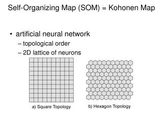
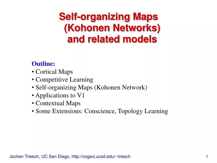
Self-organizing Maps(Kohonen Networks)and related models • Outline: • Cortical Maps • Competitive Learning • Self-organizing Maps (Kohonen Network) • Applications to V1 • Contextual Maps • Some Extensions: Conscience, Topology Learning
Optical imaging of primary visual cortex: orientation selectivity, retinal position, and ocular dominance all mapped onto 2-dim.map. Note: looks at upper layers of cortex Somatosensory System: strong magnification of certain body parts “homunculus”
General Themes Potentially high dimensional inputs are mapped onto two-dimensional cortical surface: dimensionality reduction Within one column: (from pia to white matter) similar properties of neurons Cortical Neighbors: smooth changes of properties between neighboring cortical sites In visual system: Retinotopy dominates: neighboring cortical sites process information from neighboring parts of the retina (the lower in the visual system, the stronger the effect)
Two ideas for learning mappings: • Willshaw & von der Malsburg: • discrete input and output space • all-to-all connectivity • Kohonen: • more abstract formulation • continuous input space • “weight vector” for each output
Applications of Hebbian Learning:Retinotopic Connections tectum retina Retinotopic: neighboring retina cells project to neighboring tectum cells, i.e. topology is preserved, hence “retinotopic” Question: How do retina units know where to project to? Answer: Retina axons find tectum through chemical markers, but fine structure of mapping is activity dependent
retina tectum Willshaw & von der Malsburg Model • Principal assumptions: • local excitation of neighbors in retina and tectum • global inhibition in both layers • Hebbian learning of feed-forward weights, with constraint on sum of pre-syn. weights • spontaneous activity (blobs) in retina layer • Why should we see retinotopy emerging? cooperation in intersection area instability, tectum blob can only form at X or Y competition for ability to innervate tectum area
Model Equations Weight update: Weight Normalization: M = # pre cells N = # post cells Hj* = activity in post-synaptic cell j Ai* = activity of pre-synaptic cell i, either 0 or 1 sij = connection weight from i j ekj = excitatory connection of post-synaptic cell k post-synaptic cell j ikj = inhibitory connection of post-synaptic cell k post-synaptic cell j
Retina Tectum half retina experiment Results: Systems Matching models of this type account for a range of experiments: “half retina”, “half tectum”, “graft rotation”, … Formation of retinotopic mappings
simple linear units, input is define winner: output of unit: Simple Competitive Learning Assume weights >0 and possibly weights normalized. If weights normalized, hi maximal if wi has smallest Euclidean distance to . “ultra-sparse code” Figure taken from Hertz et.al. Winner-Take-All Mechanism: may be implemented through lateral inhibition network (see part on Neurodynamics)
weight vector input vector learning rule is Hebb-like plus decay term Weight of winning unit is moved towards current input . Similar to Oja´s and Sanger´s rule. Geometric interpretation: units (their weights) move in input space. Winning unit moves towards current input. normalized weights Figure taken from Hertz et.al.
Cost function forCompetitive Learning Claim: Learning rule related to this cost function: minimization of sum of squared errors! To see this, treat M as constant: Note 1: may be seen as online version of k-means clustering Note 2: can modify learning rule to make all units fire equally often
Vector Quantization Idea: represent input by weight vector of the winner (can be used for data compression: just store/transmit label representing the winner) Question: what is set of inputs that “belong” to a unit i, i.e. for which unit i is winner? Answer: Voronitesselation (note: matlab command for this) Figure taken from Hertz et.al.
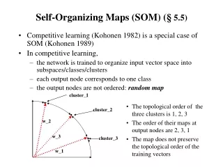
Self-Organizing Maps (Kohonen) Idea: Output units have a prioritopology (1-dim. or 2-dim.), e.g. are arranged on a chain or regular grid. Not only winner get´s to learn but also its neighbors. SOMs transform incoming signal patterns of arbitrary dimension on 1-dim. or 2-dim. map. Neighbors in the map respond to similar input patterns. Competition: again with winner-take-all mechanism Cooperation: through neighborhood relations that are exploited during learning
weight vector input vector Self-Organizing Maps (Kohonen) example of 1-dim. topology of output nodes Neighboring output units learn together! Update winner’s weights but also those of neighbors.
Usually, neighborhood shrinks with time: (for 0 : competetive learning) Define winner: Same learning rule as earlier: SOM algorithm again, simple linear units, input is Output of unit j when winner is i*: , Usually, learning rate decays, too:
2 Learning Phases time dependence of parameters: , 1. Self-organizing or ordering phase - topological ordering of weight vectors - use: = radius of layer 2. Convergence phase - fine tuning of weights - use: very small neighborhood, learning rate around 0.01
Examples Figure taken from Haykin
Feature Map Properties Property 1: feature map approximates the input space Property 2: topologically ordered, i.e. neighboring units correspond to similar input patterns Property 3: density matching: density of output units corresponds qualitatively to input probability density function. SOM tends to under-sample high density areas and over-sample low-density areas Property 4: can be thought of (loosely) as non-linear generalization of PCA.
Ocular Dominance and Orientation Tuning in V1 1. singularities (pinwheels and saddle points) tend to align with centers of ocular dominance bands 2. isoorientation contours intersect borders of ocular dominance bands at approximately 90 deg. angle (“local orthogonality”) 3. global disorder: (Mexican-hat like autocorrelation functions)
SOM based Model Obermayer et al.: SOM model and close relative (elastic net) account for observed structure of pinwheels and their locations:
Elastic Net Model Very similar idea: (Durbin and Mitchinson) Note: explicitly forces unit’s weight to be similar to that of neighbors
RF-LISSOM modelReceptive Field Laterally Interconnected Synergetically Self-Organizing Map Idea: learn RF properties and map simultaneously Figures taken from http://www.cs.texas.edu/users/nn/web-pubs/htmlbook96/sirosh/
Lissom equations input activities are elongated Gaussian blobs: initial map activity is nonlinear function of input activity, weights μ: time evolution of activity (μ, E, I are all weights): Hebbian style learning with weight normalization: all weights learn but with different parameters:
Demo: (needs supercomputer power)
Contextual Maps Different way of displaying SOM: label output nodes with a class label describing what output node represents. Can be used to display data from high dimensional input spaces in 2d. Figure taken from Haykin Input vector is concatenation of attribute vector and symbol code: (symbol code “small” and free of correlations)
Contextual Maps cont’d. Contextual Map trained just like standard SOM. Which unit is winner for symbol input only? Figure taken from Haykin
Contextual Maps cont’d. For which symbol code fires unit the most? Figure taken from Haykin
Extension with “Conscience” Problem: standard SOM does not faithfully represent input density Magnification factor: m(x) is the number of units in small volume dx of input space. Ideally: But this is not what SOM does! Idea (DeSieno): If neuron wins too often/not often enough, it decreases/increases its chance of winning. (intrinsic plasticity)
Topology Learning: neural gas idea: no fixed underlying topology but learn it on-line Figure taken from Ballard
SOM Summary • “simple algorithms” with complex behavior. • Can be used to understand organization of response preferences • for neurons in cortex, i.e. formation of cortical maps. • Used for visualization of high dimensional data. • Can be extended for supervised learning. • Some notable extensions, e.g. neural gas and growing neural gas, • that are generalizations to 2-dim topology. Proper (local) • topology is discovered during the learning process
Learning Vector Quantization Idea: supervised add-on for the case that class labels are available for the input vectors How it works: first do unsupervised learning, then label output nodes Learning rule: Cx: desired class label for input x Cw: class label of winning unit with weight vector w In case Cw=Cx: w=a(t)[x-w] (move weight towards input) In case CwCx: w=-a(t)[x-w] (move away from input) a(t): decaying learning rate Figure taken from Haykin
LVQ data:
LVQ result: Figure taken from Haykin