Download
1 / 37
730 likes | 2.35k Views
Expected Utility Theory. How to deal with uncertainty. Introduction. we have talked about individual decision making in the absence of uncertainty in reality, we usually make decision under uncertainty example: 1 . uncertainty from product quality (second-hand vehicle)

E N D
Expected Utility Theory How to deal with uncertainty
Introduction • we have talked about individual decision making in the absenceof uncertainty • in reality, we usually make decision under uncertainty • example: 1. uncertainty from product quality (second-hand vehicle) 2. uncertainty in dealing with others -> often the outcome depends on what others do 3. purchase of financial assets (stocks and bonds) whose returnis contingent on which state is realized. This is the essence of Financial Economics
2 Goals 10 0.4 E(W) = 0.4(10) + 0.6(2) = 5.2 1) Individual maximizes their expected Utility Asset i E[U(W)] = 0.4U(10) + 0.6U(2) = ? 0.6 2 Prefer the one with higher E[U(W)] 9 0.3 E(W) = 0.3(9) + 0.7(4) = 5.5 Asset j E[U(W)] = 0.3U(9) + 0.7U(4) = ? 0.7 4 2) Individual preferences over risk and return y C2 Return x C1 Risk
Probability • probability of an event occurring is the relative frequency with whichthe event occurs • if αi = the probability of event i occurringand there are n possible events (states)then • 1. αi> 0, i = 1…n • 2. αi = 1 • Lottery (X) with prizes (outcomes, states, events) • X1, X2, X3,...,Xn with corresponding probabilities • α1, α2, α3,...,αn , respectively (mutually exclusive and exhaustive) • then the expected value of this lottery is • E(X) = α1X1 + α2X2 + α3X3 + ... + αnXn • E(X) = αiXi n ‘i=1 n ‘i=1
Example 1 • Gamble (X) flip of a coin • if heads, you receive $1 X1 = +1 • if tails, you pay $1 X2 = -1 • E(X) = (0.5) (1) + (0.5) (-1) = 0 • if you play this game many times, it is likely that you break-even
Example 2 • Gamble (X) flip of a coin • if heads, you receive $10 X1 = +10 • if tails, you pay $1 X2 = -1 • E(X) = (0.5) (10) + (0.5) (-1) = 4.50 • if you play this game many times, you will be a big winner • How much would you pay to play this game: • perhaps as much as a $4.50 • But of course the answer depends upon your preference to risk
Fair Gambles • if the cost to play = expected value of these gambles the outcome • then the gamble is said to be actuarially fair • Common empirical findings: 1. individuals may agree to flip a coin for small amounts of money,but usually refuse to bet large sums of money 2. people will pay small amounts of money to play actuarially unfair games (Lotto 649, where cost = $1, but E(X) < 1) - but will avoid paying a lot Why do these empirical findings occur? Becoz’ it is not about E(W)
St. Petersburg Paradox • Gamble (X): • A coin is flipped until a head appearsYou receive $2n where n is the flip on which the head occurred • states: X1 = $2 X2 = $4 X3 = $8 ... Xn = $2n • prob: α1 = 1/2 α2 = 1/4 α3 = 1/8 ... αn = 1/2n E(X) = Paradox: no one would pay an “actuarially fair” price to play this game(no one would even pay close to the fair price)
Explaining the St. Petersburg Paradox • this paradox arises because individuals do not make decisionsbased purely on wealth, but rather on the utility oftheir expected wealth • if we can show that the marginal utility of wealthdeclines as we get more wealth, then we can show that theexpected value of a game is finite • Assume U(X) = ln(X) U'(X)=1/x > 0 MU positive • U"(X)=-1/x2 < 0 Diminishing MU • E(U(W)) = E(αi U(Xi))= (αi ln(Xi)) = 1.39 < • an individual would pay an amount up to 1.39 unitsof utility to play this gamble ‘i=1 ‘i=1
Expected Utility Theory • Objective: to develop a theory of rational decision-making under uncertainty with the minimum sets of reasonable assumptions possible • the following five axioms of cardinal utility provide the minimum setof conditions for consistent and rational behaviour • What do these axioms of expected utility mean? 1. all individuals are assumed to make completely rational decisions (reasonable) 2. people are assumed to make these rational decisions among thousandsof alternatives (hard)
5 Axioms of Choice under uncertainty A1.Comparability (also known as completeness). For the entire set of uncertain alternatives, an individual can say either that either x is preferred to outcome y (x > y) or y is preferred to x (y > x) or indifferent between x and y (x ~ y). A2.Transitivity (also know as consistency). If an individual prefers x to y and y to z, then x is preferred to z. If (x > y and y > z, then x > z). Similarly, if an individual is indifferent between x and y and is also indifferent between y and z, then the individual is indifferent between x and z. If (x ~ y and y ~ z, then x ~ z).
5 Axioms of Choice under uncertainty A3.Strong Independence. Suppose we construct a gamble where the individual has a probability α of receiving outcome x and a probability (1-α) of receiving outcome z. This gamble is written as: G(x,z:α) Strong independence says that if the individual is indifferent to x and y, then he will also be indifferent as to a first gamble set up between x with probability α and a mutually exclusive outcome z, and a second gamble set up between y with probability α and the same mutually exclusive outcome z. If x ~ y, then G(x,z:α) ~ G(y,z:α) NOTE: The mutual exclusiveness of the third outcome z is critical to the axiom of strong independence.
5 Axioms of Choice under uncertainty A4.Measurability. (CARDINAL UTILITY) If outcome y is less preferred than x (y < x) but more than z (y > z), then there is a unique probability α such that: the individual will be indifferent between [1] y and [2] A gamble between x with probability α z with probability (1-α). In Maths, if x > y > z or x > y > z , then there exists a unique α such that y ~ G(x,z:α)
5 Axioms of Choice under uncertainty A5.Ranking. (CARDINAL UTILITY) If alternatives y and u both lie somewhere between x and z and we can establish gambles such that an individual is indifferent between y and a gamble between x (with probability α1) and z, while also indifferent between u and a second gamble, this time between x (with probability α2) and z, then if α1 is greater than α2, y is preferred to u. If x > y > z and x > u > z then if y ~ G(x,z:α1) and u ~ G(x,z:α2), then it follows that if α1 > α2 then y > u, or if α1 = α2, then y ~ u
One more assumption • People are greedy, prefer more wealth than less. • The 5 axioms and this assumption is all we need in order to develop a expected utility theorem and actually apply the rule of max E[U(W)] = max ∑iαiU(Wi)
Utility Functions • Utility functions must have 2 properties 1. order preserving: if U(x) > U(y) => x > y 2. Expected utility can be used to rank combinations of risky alternatives: U[G(x,y:α)] = αU(x) + (1-α) U(y) • Deriving Expected utility theorem, one of the most elegant derivations in Economics, is tough. Don’t worry about a formal derivation. Just apply it. • Remark: Utility functions are unique to individuals - there is no way to compare one individual's utility function with another individual's utility - interpersonal comparisons of utility are impossible if we give 2 people $1,000 there is no way to determine who is happier
One more element: Risk Aversion • Consider the following gamble: • Prospect a prob = α G(a,b:α) • prospect b prob = 1-α • Question: Will we prefer the expected value of the gamble with certainty, or will we prefer the gamble itself? • ie. consider the gamble with • 10% chance of winning $100 • 90% chance of winning $0 E(gamble) = $10 • would you prefer the $10 for sure or would you prefer the gamble? if prefer the gamble, you are risk loving if indifferent to the options, risk neutral if prefer the expected value over the gamble, risk averse
Preferences to Risk U(W) U(W) U(W) U(b) U(b) U(a) U(b) U(a) U(a) a b W a b W a b W Risk Preferring Risk Neutral Risk Aversion U'(W) > 0 U''(W) = 0 U'(W) > 0 U''(W) > 0 U'(W) > 0 U''(W) < 0
The Utility Function U(W) 3.40 3.00 Let U(W) = ln(W) U'(W) > 0 U''(W) < 0 U'(W) = 1/w U''(W) = - 1/W2 MU positive But diminishing 2.30 1.61 0 W 1 5 10 20 30
U[E(W)] and E[U(W)] • U[(E(W)] is the utility associated with the known level of expected wealth (although there is uncertainty around what the level of wealth will be, there is no such uncertainty about its expected value) • E[U(W)] is the expected utility of wealth is utility associated with level of wealth that may obtain • The relationship between U[E(W)] and E[U(W)] is very important
Expected Utility • Assume that the utility function is natural logs: U(W) = ln(W) • Then MU(W) is decreasing • U(W) = ln(W) • U'(W)=1/W • MU>0 • MU''(W) < 0 => MU diminishing Consider the following example: 80% change of winning $5 20% chance of winning $30 E(W) = (.80)*(5) + (0.2)*(30) = $10 U[E(W)] = U(10) = 2.30 E[U(W)] = (0.8)*[U(5)] + (0.2)*[U(30)] = (0.8)*(1.61) + (0.2)*(3.40) = 1.97 Therefore, U[(E(W)] > E[U(W)] -- uncertainty reduces utility
The Markowitz Premium U(W) 3.40 U(W) = ln(W) U[E(W)] = U(10) = 2.30 E[U(W)] = 0.8*U(5) + 0.2*U(30) = 0.8*1.61 + 0.2*3.40 = 1.97 Therefore, U[E(W)] > E[U(W)] Uncertainty reduces utility Certainty equivalent: 7.17 That is, this individual will take 7.17 with certainty rather than the uncertainty around the gamble U[E(W)] = 2.30 E[U(W)] = 1.97 1.61 2.83 0 W 1 5 CE = 7.17 10 30
The Certainty Equivalent • The Expected wealth is 10 • The E[U(W)] = 1.97 • How much would this individual take with certainty and be indifferent the gamble • Ln(CE) = 1.97 • Exp(Ln(CE)) = CE = 7.17 • This individual would take 7.17 with certainty rather than the gamble with expected payoff of 10 • The difference, (10 – 7.17 ) = 2.83, can be viewed as a risk premium – an amount that would be paid to avoid risk
The Risk Premium • Risk Premium: • the amount that the individual is willing to give up in order to avoid the gamble • Recall the gamble 80% change of winning $5 20% chance of winning $30 E(W) = (.80)*(5) + (0.2)*(30) = $10 Suppose the individual has the choice now between the gamble and the expected value of the gamble E[U[W)] = 1.97 Certainty equivalent = $7.17 Investor would be willing to pay a maximum of $2.83 to avoid the gamble ($10 - $7.17) ie will pay an insurance premium of $2.83. THIS IS CALLED THE MARKOWITZ PREMIUM Ln(CE)=1.97, i.e U(CE)=E[U(W)], CE=7.17, RP=10-7.17=$2.83
The Risk Premium Risk Premium = an individual's expected wealth,given he plays the gamble - level of wealth the individual would accept with certainty if the gamble were removed (ie the certainty equivalent) In general, if U[E(W)] > E[U(W)] then risk averse individual (RP > 0) if U[E(W)] = E[U(W)] then risk neutral individual (RP = 0) if U[E(W)] < E[U(W)] then risk loving individual (RP < 0) risk aversion occurs when the utility function is strictly concave risk neutrality occurs when the utility function is linear risk loving occurs when the utility function is convex
The Arrow-Pratt Premium • Risk Averse Investors • assume that utility functions are strictly concave and increasing • Individuals always prefer more to less (MU > 0) • Marginal utility of wealth decreases as wealth increases • A More Specific Definition of Risk Aversion • W = current wealth • gamble Z and the gamble has a zero expected value • E(Z) = 0 • what risk premium (W,Z) must be added to the gamble to make the individual indifferent between the gamble and the expected value of the gamble?
The Arrow-Pratt Premium The risk premium can be defined as the value that satisfies the following equation: E[U(W + Z)] = U[ W + E(Z) - ( W , Z)] (*) LHS: RHS: expected utility of utility of the current level of wealth the current level plus of wealth, given the the expected value of gamble the gamble less the risk premium We want to use a Taylor series expansion to (*) to derive an expression for the risk premium (W,Z)
Absolute Risk Aversion • Arrow-Pratt Measure of a Local Risk Premium (derived from (*) above) • define ARA as a measure of Absolute Risk Aversion • this is defined as a measure of absolute risk aversion because itmeasures risk aversion for a given level of wealth • ARA > 0 for all risk averse investors (U'>0, U''<0) • How does ARA change with an individual's level of wealth? • ie. a $1000 gamble may be trivial to a rich man, but non-trivial to apoor man => ARA will probably decrease as our wealth increases
Relative Risk Aversion • Constant RRA => An individual will have constant risk aversion to a "proportional loss" of wealth, even though the absolute loss increases as wealth does • Define RRA as a measure of Relative Risk Aversion
Quadratic Utility Quadratic Utility - widely used in the academic literature U(W) = a W - b W2 U'(W) = a - 2bW U"(W) = -2b -U"(W) 2b ARA = --------- = --------- U'(W) a -2bW d(ARA) ------- > 0 dW 2b RRA = --------- a/W - 2b d(RRA) ------- > 0 dW quadratic utility exhibits increasing ARA and increasing RRA ie an individual with increasing RRA would become more averse to a given percentage loss in W as W increases - not intuitive
The Empirical Evidence • Empirical evidence (Friend and Blume (1975)) indicates that individuals have decreasing ARA and constant RRA = 2 • Power Utility Function U(W) = -W-1 U'(W) = W-2 > 0 U"(W) = -2W-3 < 0 ARA = 2/W => dARA/dW < 0 RRA = 2W/W = 2 => dRRA/dW = 0 This power utility function is consistent with the empirical evidence of Friend and Blume (1975) U(W) = -1/W
An Example • U=ln(W) W = $20,000 • G(10,-10: 50) 50% will win 10, 50% will lose 10 • What is the risk premium associated with this gamble? • Calculate this premium using both the Markowitz and Arrow-Pratt Approaches
Arrow-Pratt Measure • = -(1/2) 2z U''(W)/U'(W) • 2z = 0.5*(20,010 – 20,000)2 + 0.5*(19,090 – 20,000)2 = 100 • U'(W) = (1/W) U''(W) = -1/W2 • U''(W)/U'(W) = -1/W = -1/(20,000) • = -(1/2) 2z U''(W)/U'(W) = -(1/2)(100)(-1/20,000) = $0.0025
Markowitz Approach • E(U(W)) = piU(Wi) • E(U(W)) = (0.5)U(20,010) + 0.5*U(19,990) • E(U(W)) = (0.5)ln(20,010) + 0.5*ln(19,990) • E(U(W)) = 9.903487428 • ln(CE) = 9.903487428 CE = 19,999.9975 • The risk premium RP = $0.0025 • Therefore, the AP and Markowitz premia are the same
Markowitz Approach E(U(W)) = 9.903487 20,010 19,990 20,000 CE
Differences in two approaches • Markowitz premium is an exact measures whereas the AP measure is approximate • AP assumes symmetry payoffs across good or bad states, as well as relatively small payoff changes. • It is not always easy or even possible to invert a utility function, in which case it is easier to calculate the AP measure • The accuracy of the AP measures decreases in the size of the gamble and its asymmetry
Mean & Variance as choice variables • With 5 axioms, prefer more to less, we have Expected utility theorem • With risk-aversion assumption, we solve St. Petersburg’s paradox • With returns of risky assets being jointly normally distributed, we can draw indifference curves on the plane of return (E(r)) and risk (var(r) or standard deviation of r) as the right diagram • Essentially, mean and variance are the choice variables investors concern about in order to max their E[U(w)] Return Risk