Download
1 / 35
350 likes | 444 Views
Multi-Lag Cluster Enhancement of Fixed Grids for Variogram Estimation for Near Coastal Systems . Kerry J. Ritter, SCCWRP Molly Leecaster, SCCWRP N. Scott Urquhart, CSU Ken Schiff , SCCWRP Dawn Olsen, City of San Diego Tim Stebbins, City of San Diego. Project Funding.

E N D
Multi-Lag Cluster Enhancement of Fixed Grids for Variogram Estimation for Near Coastal Systems Kerry J. Ritter, SCCWRP Molly Leecaster, SCCWRP N. Scott Urquhart, CSU Ken Schiff , SCCWRP Dawn Olsen, City of San Diego Tim Stebbins, City of San Diego
Project Funding • The work reported here was developed under the STAR Research Assistance Agreement CR-829095 awarded by the U.S. Environmental Protection Agency (EPA) to Colorado State University. This presentation has not been formally reviewed by EPA. The views expressed here are solely those of the presenter and STARMAP, the Program they represent. EPA does not endorse any products or commercial services mentioned in this presentation. • Southern Californian Coastal Water Research Project (SSCWRP)
Background • Maps of sediment condition are important for making decisions regarding pollutant discharge • Maps in marine systems are rare • Special study by San Diego Municipal Wastewater Treatment Plant • Objective: To build statistically defensible maps of chemical constituents and biological indices around two sewage outfalls • Point Loma • South Bay
TYPICAL DESIGN SITUATION • Many features of the real situation are unknown. • Here: The nature of the semivariogram • Multiple Responses • What is a good solution for one response may not be a good design for another! • Time constraint • Answer was required by June 14, 2004
Two-Phase Approach • Phase I: Model spatial variability at various spatial scales (eg. Variogram) • This summer • Phase II: Use information from Phase I to design survey that meets accuracy requirements • next summer = 2005 • Current focus is on Phase I
Variogram SILL=> RANGE } NUGGET=>
Design Considerations for Modeling the Variogram • Sufficient replication at various spatial scales • Variogram model • Parameter estimates • Adequate spatial coverage to support investigating • Stationarity • Isotropy vs. Anisotropy • Strata • Allow for multiple responses
Multi-Lag Cluster (MCL) Enhancements to Fixed Grids • Clusters of sites, spaced at various lag distances, are placed around fixed locations on an existing grid. • Allows current monitoring grid to remain “in tact”. • Provides replication at multiple spatial-scales
There are many ways to allocate resources within the MLC • Economic constraints: limit total number of samples • ( eg. 100 in Point Loma) • More clusters with fewer sites within a cluster? • or less clusters with fewer sites? • Shorter sample spacing or larger sample spacing? • What is best (decent!) design configuration?
Choosing the Best DesignCase Study: Point Loma • Three design configurations • S, STAR, and S with satellites • Two sets of lag classes • Shorter vs. larger sample spacing • Compare lag distributions • Simulation study • Simulate response • Consider different models of spatial variability • Compare relative performance of designs for estimating parameters
“S” Cluster Design Lag = 0.05, 0.10, 0.20, 0.50 Lag = 0.05, 0.25, 1.00, 3.00
Omnidirectional Lag Dist. Lag = 0.05, 0.25, 1.00, 3.00 Lag = 0.05, 0.10, 0.20, 0.50
Directional Lag DistLag = 0.05, 0.10, 0.20, 0.50{ Lag = 0.05, 0.25, 1.00, 3.00 is similar}
Simulation Study 3 Grid Enhancements: S, STAR, S with Satellites Two sets of lag classes of size 4 0.05, 0.10, 0.20, 0.50 (km) 0.05, 0.25, 1, 3 (km) Spherical variogram Range = 1, 2, 4, 6 Nugget = 0.00, 0.10 Sill = 1 1000 sims Fit using automated procedure in Splus This may have introduced artifacts
Percent Difference from Target Range(Median Range) S=1, N= 0.10 Lag = 0.05, 0.10, 0.20, 0.50 Lag = 0.05, 0.25, 1.00, 3.00
Percent Difference from Target Sill(Median Sill) S=1, N= 0.10 Lag = 0.05, 0.10, 0.20, 0.50 Lag = 0.05, 0.25, 1.00, 3.00
Percent Difference from Target Nugget(Median Nugget) S=1, N= 0.10 Lag = 0.05, 0.10, 0.20, 0.50 Lag = 0.05, 0.25, 1.00, 3.00
Summary STAR- performed better than S and S with Satellites for estimating variogram parameters - robust to different lag classes Multiple lag distances better than increased replication at fewer lag distances Larger lag classes generally did better than shorter lag classes (eliminates “holes”)
Final Design Five “S” clusters and includes10 duplicates: five at star centers & five elsewhere)
Further Research • Choose another variogram model • Exponential • Choose another variogram fitting algorithm • REML • Simulate anisotropy • Investigate robustness to model misspecification • Explore other designs
STARMAP and CITY OF SAN DIEGO? • Outreach to a member of the EPA affiliates • Research opportunity – real problem • Mapping consequences • Apparently no other US data exists which is • spatially intense and • near coastal • This mapping requirement resulted from SD’s permit renewal • Similar repeats are very likely
MORE GENERAL QUESTION • How much spatial correlation is there in aquatic systems, after accounting for habitat features? • I am trying to assemble spatially intense relevant data sets in a number of settings • Ask for such data sets at EMAP 2004 Symposium in May • Have located a few
SPATIALLY INTENSE DATA SETSOF ENVIRONMENTAL RESPONSES • Ohio River • Have 400+ sites • Josh French is looking at this data • Have about 60 Virginia stream sites • On two streams • Access to a northeast estuary study 100+ points • Some spatial correlation demonstrated • Detroit River – fairly short segment 60+ points • San Diego study = near coastal
SPATIALLY INTENSE DATA SETSOF ENVIRONMENTAL RESPONSES • Have nothing on wetlands • Other possibilities • San Francisco Bay • Preliminary observation – SD data shows greater range in the semivariogram than I had expected • Even after accounting for depth or particle size • Why had I expected that? Effluent is fresh water; it rises fast from outfall. Coastal and tidal currents are strong there.
END OF PLANNED PRESENTATION • Questions and suggestions are welcome