Download
1 / 25
250 likes | 362 Views
Graph Balancing. Scheduling on Unrelated Machines. M1. M3. M2. J1. J2. J3. J4. J5. Scheduling on Unrelated Machines. M1. M3. M2. J1. J1. J2. J2. J3. J3. J4. J4. J5. J5. Scheduling on Unrelated Machines. M1. J2. J3. M2. J4. J5. M3. J1. Makespan.

E N D
Scheduling on Unrelated Machines M1 M3 M2 J1 J2 J3 J4 J5
Scheduling on Unrelated Machines M1 M3 M2 J1 J1 J2 J2 J3 J3 J4 J4 J5 J5
Scheduling on Unrelated Machines M1 J2 J3 M2 J4 J5 M3 J1 Makespan
Restricted Assignment M1 M2 M3 J1 J2 J3 J4 J5
Graph Balancing • Special case of Restricted Assignment • Each job can be scheduled on at most 2 machines • Machines vertices • Jobs edges • Assign dedicated loads to vertices • Problem is to orient the edges
Graph Balancing 6 2 2 2 6 5 1 2 4 5 3 2 5 5 1 1 2
Graph Balancing Summary • Given: weighted multigraph (V, E, p, q) • V : Vertices Machines • E : Edges Jobs • eE, pe = processing time of job e • vV, qv = dedicated load on vertex v • Output: Orientation of edges :E V such that (e) e • Loadv = qv + e:v = (e) pe • Objective: Minimize maximum load
Optimization Decision Problem • -relaxed decision procedure • Is there any orientation with maximum load at most d ? • Answer: • “NO” • Orientation with maximum load at most d. • Binary search for d and scale everything appropriately
2-approximation LP • Find values xev 0, for each e and ve, such that • For each e E, u,ve: xeu + xev = 1 • For each v V: qv + e:vexevpe 1
2-Relaxed Decision Procedure • Solve LP in polynomial time. • If not feasible, return “NO” • If feasible, round solution using rotation and tree assignment • After rounding, the maximum load is at most 2 • For rounding, decompose the graph as • Cycles • Trees
Rotation .125 1/4 .5 .15 .5 1/4 .6 .3 1/2 .1 .7 .4 .5 .4 .25 1/3 1/2 .5 .6 .6 .2 .4 1/2 .3
Rotation 1/4 .1 .9 1/4 1 .1 1/2 .9 0 .3 .7 1/3 1/2 .7 .3 .4 .6 1/2
Rotation • Increases the number of integral solutions. • Breaks the fractional cycles. • Unchanged after rotation • (xeu + xev) for all edges e • (e:v e xevpe) for all vertices v • Maximum load after rotation is 1. • After all fractional cycles are broken, only fractional trees remain
Tree Assignment 1 1 1 1 1 1 1 1 1 1 1 1 1
Tree Assignment 2 1 2 1 1 2 1 1 1 2 2 1 2
Integrality Gap v` 1 1 1 1 1 1 1 1
Big edges ) 1/2 1/2 1/2 1/2 1/2 1/2 1/2
Big trees constraint 1/2 >1/2 >1/2 >1/2 1/2 1/2 1
1.75-approximation • Find values xev 0, for each e and ve, such that • For each e E, u,v e: xeu + xev = 1 • For each v V: qv + e:v e xevpe 1 • For each T GB(graph induced on big edges) 1
Algorithm 1/2 >1/2 .1 >1/2 .9 1 .1 v >1/2 1/2 .9 0 1/2 .3 v .7 .7 .3 .4 .6
Invariants • At any stage of iteration: • . • If is incident to any edge in . • If is incident to any big edge in . • Big tree constraint is not violated.
Algorithm Case 1: e is a big edge (pe >= 0.5) Increase in load = pe – xevpe= xeupe<= 0.75 Case 2: e is not a big edge (pe < 0.5) Increase in load = pe – xevpe< pe < 0.5 Since xeupe > 0.75, e is definitely a big edge For any vertex u’ in the tree T, the path joining u’ to v is also a subtree of GB By the tree constraint, xevpe + xe’u’pe’ >= pe + pe’ -1 pe’ – xe’u’pe’ <= 1 – (pe - xevpe) Increase in load <= 0.25
Integrality gap .25 .25 .25 .25 v` 1 1 1 1 .25 .25 .25 .25 .25 .25 v` 1 1 1 1 .25 .25 .25 .25 1 .25 .25 1 .25 .25 v` 1 1 .25 .25