Download
1 / 11
110 likes | 218 Views
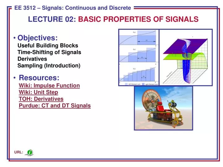
LECTURE 02: BASIC PROPERTIES OF SIGNALS. Objectives: Useful Building Blocks Time-Shifting of Signals Derivatives Sampling (Introduction) Resources: Wiki: Impulse Function Wiki: Unit Step TOH: Derivatives Purdue: CT and DT Signals. URL:. Introduction.

E N D
LECTURE 02: BASIC PROPERTIES OF SIGNALS • Objectives:Useful Building BlocksTime-Shifting of SignalsDerivativesSampling (Introduction) • Resources:Wiki: Impulse FunctionWiki: Unit StepTOH: DerivativesPurdue: CT and DT Signals URL:
Introduction • An important concept in signal processing is the representation of signals using fundamental building blocks such as sinewaves (e.g., Fourier series) and impulse functions (e.g., sampling theory). • Such representations allow us to gain insight into the complexity of a signal or approximate a signal with a lower fidelity version of itself (e.g., progressively scanned jpeg encoding of images). • In today’s lecture we will investigate some simple signals that can be used as these building blocks. • We will also discuss some basic properties of signals such as time-shifting and basic operations such as integration and differentiation. • We will learn how to represent continuous-time (CT) signals as a discrete-time (DT) signal by sampling the CT signal.
The Impulse Function • The unit impulse, also known as a Delta function or a Dirac distribution, is defined by: • The impulse function can be approximated by a rectangular pulse with amplitude A and time duration 1/A. • For any real number, K: • This is depicted to the right. • The definition of an impulse for a DT signal is: • Note that: 1/Δ t Δ K t
The Unit Step and Unit Ramp Functions • We can define a unit step function as the integral of the unit impulse function: • This can be written compactly as: • Similarly, the derivative of a unit stepfunction is a unit impulse function. • We can define a unit ramp function as theintegral of a unit step function: t
The DT Unit Step and Unit Ramp Functions • We can sum a DT unit pulse to arrive at aDT unit step function: • We can define a time-limited pulse, often referredto as a discrete-time rectangular pulse: • We can sum a unit step to arrive atthe unit ramp function:
Sinewaves and Periodicity • Sine and cosine functions are of fundamental importance in signalprocessing. Recall: • A sinusoid is an example of aperiodic signal: • A sinusoid is period with a periodof T = 2π/ω: • Later we will classify a sinewave as a deterministic signal because its values for all time are completely determined by its amplitude, A, is frequency, ω, and its phase, Θ. • Later, we will also decompose signals into sums of sins and cosines using a trigonometric form of the Fourier series.
Time-Shifted Signals • Given a CT signal, x(t), a time-shifted version of itself can be constructed:x(t-t1) delays the signal (shifts it forward, or to the right, in time), and x(t+t1), which advances the signal (shifts it to the left). • We can define the sifting property of a time-shifted unit impulse: • We can easily prove this by noting: • and:
Continuous and Piecewise-Continuous Signals • A continuous-time signal, x(t), is discontinuous at a fixed point, t1,if where are infinitesimal positive numbers. • A signal is continuous at the point if . • If a signal is continuous for all points t, x(t) is said to be a continuous signal. • Note that we use continuous two ways: continuous-time signal and continuous (as a function of t). • The ramp function, r(t), and the sinusoid are examples of continuous signals, as is the triangular pulse shown to the right. • A signal is said to bepiecewise continuousif it is continuous at allt except at a finite orcountably infinite collection of pointsti,i= 1, 2, 3, …
Derivative of a Continuous-Time Signal • A CT signal, x(t), is said to be differentiable at a fixed point, t1, ifhas a limit as h 0: • independent of whether h approaches zero from h> 0 or h< 0. • To be differentiable at a point t1, it is necessary but not sufficient that the signal be continuous at t1. • Piecewise continuous signals are not differentiable at all points, but can have a derivative in the generalized sense: • is the ordinary derivative of x(t) at all t, except at t= t1. is an impulse concentrated a t= t1 whose area is equal to the amount the function “jumps” at the point t1. • For example, for the unit step function,the generalized derivative of is:
DT Signals: Sampling • One of the most common ways in which discrete-time signals arise is sampling of a continuous-time signal. • In this case, the samples are spaced uniformly at time intervals where T is the sampling interval, and 1/T is the sample frequency. • Samples can be spaced uniformly, as shown to the right, or nonuniformly. • We can write this conveniently as: • Later in the course we will introduce the Sampling Theorem that defines the conditions under which a CT signal can be recovered EXACTLY from its DT representation with no loss of information. • Some signals, particularly computer generated ones, exist purely as DT signals.
Summary • Representation of signals using fundamental building blocks can be a useful abstraction. • We introduced four very important basic signals: impulse, unit step, ramp and a sinewave. Further we introduced CT and DT versions of these. • We introduced a mathematical representation for time-shifting a signal, and introduced the sifting property. • We discussed the concept of a continuous signal and noted that many of our useful building blocks are discontinuous at some point in time (e.g., impulse function). Further DT signals are inherently discontinuous. • We introduced the concept of a derivative of a continuous signal and noted that the derivative of a discrete-time signal is a bit more complicated. • Finally, we presented some introductory material on sampling.