Bayesian Analysis of X-ray Luminosity Functions A. Ptak (JHU)

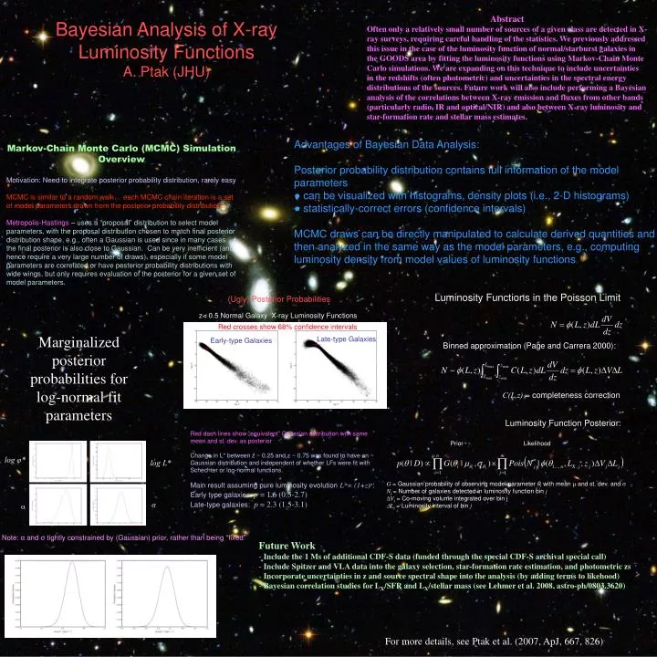
1. (Ugly) Posterior Probabilities z< 0.5 Normal Galaxy X-ray Luminosity Functions Red crosses show 68% confidence intervals Late-type Galaxies Early-type Galaxies Abstract Often only a relatively small number of sources of a given class are detected in X-ray surveys, requiring careful handling of the statistics. We previously addressed this issue in the case of the luminosity function of normal/starburst galaxies in the GOODS area by fitting the luminosity functions using Markov-Chain Monte Carlo simulations. We are expanding on this technique to include uncertainties in the redshifts (often photometric) and uncertainties in the spectral energy distributions of the sources. Future work will also include performing a Bayesian analysis of the correlations between X-ray emission and fluxes from other bands (particularly radio, IR and optical/NIR) and also between X-ray luminosity and star-formation rate and stellar mass estimates. Bayesian Analysis of X-ray Luminosity Functions A. Ptak (JHU) Advantages of Bayesian Data Analysis: Posterior probability distribution contains full information of the model parameters ●can be visualized with histograms, density plots (i.e., 2-D histograms) ● statistically-correct errors (confidence intervals) MCMC draws can be directly manipulated to calculate derived quantities and then analyzed in the same way as the model parameters, e.g., computing luminosity density from model values of luminosity functions Markov-Chain Monte Carlo (MCMC) Simulation Overview Motivation: Need to integrate posterior probability distribution, rarely easy MCMC is similar to a random walk… each MCMC chain iteration is a set of model parameters drawn from the posterior probability distribution. Metropolis-Hastings – uses a “proposal” distribution to select model parameters, with the proposal distribution chosen to match final posterior distribution shape, e.g., often a Gaussian is used since in many cases the final posterior is also close to Gaussian. Can be very inefficient (and hence require a very large number of draws), especially if some model parameters are correlated or have posterior probability distributions with wide wings, but only requires evaluation of the posterior for a given set of model parameters. Luminosity Functions in the Poisson Limit Marginalized posterior probabilities for log-normal fit parameters Binned approximation (Page and Carrera 2000): C(L,z) = completeness correction Luminosity Function Posterior: Red dash lines show “equivalent” Gaussian distribution with same mean and st. dev. as posterior Change in L* between z ~ 0.25 and z ~ 0.75 was found to have an ~ Gaussian distribution and independent of whether LFs were fit with Schechter or log-normal functions. Main result assuming pure luminosity evolution L*(1+z)p: Early type galaxies: p = 1.6 (0.5-2.7) Late-type galaxies: p = 2.3 (1.5-3.1) Prior Likelihood log φ* log L* G = Gaussian probability of observing model parameter θi with mean and st. dev. and  Nj = Number of galaxies detected in luminosity function bin j Vj= Co-moving volume integrated over bin j Lj= Luminosity interval of bin j s a Note: α and σ tightly constrained by (Gaussian) prior, rather than being “fixed” • Future Work • Include the 1 Ms of additional CDF-S data (funded through the special CDF-S archival special call) • Include Spitzer and VLA data into the galaxy selection, star-formation rate estimation, and photometric zs • Incorporate uncertainties in z and source spectral shape into the analysis (by adding terms to likehood) • Bayesian correlation studies for LX/SFR and LX/stellar mass (see Lehmer et al. 2008, astro-ph/0803.3620) For more details, see Ptak et al. (2007, ApJ, 667, 826)