Download
1 / 20
210 likes | 393 Views
On the coherency of Value at Risk ( VaR ). Roy Endré Dahl University of Stavanger. IAEE Conference Stockholm 22.06.2011. Outline. Introduction to Value at Risk ( VaR ) Motivation Define subadditivity violation Empirical results Conclusion References. Value at Risk ( VaR ).

E N D
On the coherency of Value at Risk (VaR) Roy Endré DahlUniversity of Stavanger IAEE Conference Stockholm 22.06.2011
Outline • Introduction to Value at Risk (VaR) • Motivation • Definesubadditivityviolation • Empiricalresults • Conclusion • References
Value at Risk (VaR) • One of the most common approaches to estimate portfolio risk in the energy industry as well as most other industries is Value at Risk (VaR). • VaR defines the worst case scenario within a certain confidence level over a specified time horizon (Jorion, 2001). This introduces the two parameters of a VaR: its confidence level and time horizon. • VaR can be defined by asking a simple question: How much is it possible to lose within a certain time period at a certain significance level? • E.g.: For the next day (period) 1% (significance level) of losses will be bigger than 500k (VaR). Or: I am 99% (confidence level) certain that my losses will not be bigger than 500k (VaR) the next day (period).
VaRestimationmethods • Analyticalapproach • Estimatesunderlyingdistributions. • Monte Carlo simulation • More freedomwith parameters adjustingtheestimate. • Historicalsimulation • Usesempiricaldistributiondirectly – does not needanyassumptionsondistribution.
Previous studies • Coherency • Artzner et al. (1997 and 1999)Characterized a coherent risk measure by 4 criteria, and proved that VaR is not coherent, as it violates subadditivity. • Markowitz (1959)Portfolio theoryand diversification. • Development of coherent alternatives • Artzner et al. (1999)Worst conditional expectation and tail conditional expectation. • Rockafellar and Uryasev (2000); Acerbi and Tasche (2002)Expected shortfall or conditional VaR. • Embrechts et al. (2002); Embrechts, Neslehova and Wüthrich (2009)Using copulas when estimating VaR. • Further analysis of none coherency and the implications • Danielsson et al. (2005); Ibragimov (2007)Considers the implications of violating subadditity theoretically, and concludes that if the degree of freedom is less or equal to 1, there is a risk of violations. • The financial crisis • Basel Accord II – a regulative for the financial sector to control risk. • FSA (2009)Conclude that VaR estimates in the build-up to the financial crisis was too optimistic, and recommends implementing fatter tails (more uncertainty) into the estimations.
Definesubadditivityviolation • The lackofsubadditivitycan be proven by definingsomekeynotations: • PositionVaR(∙)A position VaR is defined as the VaR for the asset, e.g. for asset A, the position VaR = VaR(A). • Contribution VaR(∙) Given a portfolio with two assets A and B, the contribution VaR for B is defined as the VaR for the portfolio VaR subtracted by the VaR for the portfolio without asset B.
Definesubadditivityviolation (2) • Diversification.According to general portfolio theory, diversification ensures that the risk in a portfolio of two assets is lower than the sum of the risk from two individual assets: • And thus: • Therefore VaRguarantees diversification (and subadditivity) if the following is provided:
Consequencesofsubadditivityviolation • Incentive to split portfolio into sub-portfolios, in order to reduce risk. For the financial sector following the Basel Accords, this would reduce the required amount of capital reserve, but without the guarantee of reduced risk. • May misguide the portfolio manager, since some risk may be hidden as a result of subbaditivity violation. • Problem for regulators, since a portfolio manager may purposely reduce risk by dividing portfolios, and representing the sum as the combined risk.
Motivation • Although previous studies suggest that only portfolios where the return on underlying risk factors are highly uncertain (degree of freedom <= 1), subadditivity violations can still occur when using historical simulation. • This paper studies the risk of subadditivity violation empirically by using S&P stock data and oil market data. • The paper also includes a theoretical comparison to student’s t generated data through a Monte Carlo simulation.
Violation using historical simulation • The historical estimation uses the historical data directly by using actual changes as the possible outcomes of the coming change. If the historical data comprise of 201 days, the 200 possible changes together constitute the distribution of tomorrow’s change. By sorting the outcomes VaR can be easily found as the 2nd worst scenario for a 99% VaR level. • The example below show how VaR may violate subadditivity. Contribution VaR(A) = 7 800 – 400 = 7 400 > 7 000 =Position VaR (A)
Monte Carlo study with high degrees of freedom • The Monte Carlo study uses the notion of position VaR and contribution VaR in order to confirm the findings in Danielsson et al. (2005). In addition, the test is carried out with bigger portfolios (N=10 and N=100). • The first part (N=2) confirms the findings in Danielsson. When the tail is extreme (degree of freedom = 1) the violations occur at 50% of the time. With thinner tails (df > 1) the risk of subadditivity is none-existent. • However, when increasing the number of assets in a portfolio, the number of subadditivity violations become negligible, even with extreme tails (df = 1). • This suggests that lack of subadditivity is just a special case problem. • The results are regardless of VaR level.
Empirical analysis S&P • The S&P data series include 10 years (10.10.2000 – 05.10. 2010) with more than 400 stocks traded on a daily basis. • The stocks are studied over several portfolios. S&P 500 stocks are studied using industry portfolios and a more general portfolio is comprised of the S&P 100 stocks. • Volatility (standard deviation of log-return) shows that the data covers a relatively calm period and a shift at the end of the period during the financial crisis.
Empirical analysis S&P • The S&P data series are positively correlated, and experiences several concurrent negative extreme events. • Extreme event is defined as a 1% probable event. • On average 4.66% of the time, more than 25% of the assets in any of the S&P portfolios concurrently experience an extreme event S&P 500 Energy S&P 500 Financials S&P 500 IT
Empirical analysis S&P • Even though the analysis show that the data involves fat tails, there is tail dependence suggesting higher correlation in the tail and the possibility of tail coarseness, the empirical analysis of S&P data concludes that the risk of subadditivity violations is none-existent.
Empiricalanalysisoil market • While previous studies support the use of historical simulation as an adequate risk estimation method for a portfolio containing stocks from the S&P 500 during the financial crisis (Dahl, 2011), • The oil market is more volatile in general (Hamilton, 2009), and historical simulation has been proved to be too optimistic during shifts like the one seen during the financial crisis Dahl and Asche (2010). • This suggests that the risk of subadditivity violations is higher because of fatter tails.
Empiricalanalysisoil market • The oil market data series include 8 years (01.10.2002 – 10.09.2009) and includes 7 oil products. • The volatility is relatively calm in the beginning of the period, but in the build-up to and during the financial crisis the volatility is extreme. • The data is more positively correlated than the S&P data, which is also confirmed when considering concurrent extreme events, where 25% of the products experience extreme events on the same date 27% of the time. Oil market portfolio
Empiricalanalysisoil market • The oil products are tested in several portfolios, and for portfolios only consisting of 2 products, there is some risk of violating subadditivity. • However, the risk is very small and negligible for both VaR levels. • When combining more than 2 products in a portfolio, violations do not occur.
Conclusion • Although considered the Achilles’ heel of VaR, the lack of subadditivity is not a practical problem. • Further studies should be concentrated on finding more efficient and accurate estimates, and not trying to find methods that fulfil the coherency criteria. • When using historical simulation, special care should be taken to avoid tail coarseness. • Also, increased dependency in the tail region can be solved by using copulas with VaR (Embrechts, 2009).
References • Acerbi, C. and D. Tasche. ”On thecoherencyofExpectedShortfall” // Journal of Banking and Finance, 26(7), 1487 – 1503, 2002. • Asche, F. and R. E. Dahl. ”MultivariateStudent’s t Monte Carlo EstimationofValue-At-Risk in energyportfolio.” // IAEE Vilnius Proceedings, 2010. • Artzner, P., F. Delbaen, J-M Eber and D. Heath. ”ThinkingCoherently” // RISK, 10, 68-71, 1997. • Artzner, P., F. Delbaen, J-M Eber and D. Heath. ”CoherentMeasuresof Risk” // Mathematical Finance, 9, 203-228, 1999. • Dahl, R. E. ”Whyhistoricalsimulationworks – EmpiricalstudyofValue-At-Risk in S&P 500 during thefinancialcrisis.” // Workingpaper, University of Stavanger, 2011. • Danielsson, J., B. N. Jorgensen, S. Mandira, G. Samorodnitksy and C. G. de Vries. ”SubadditivityRe-Examined: the Case ofValue-at-Risk” // FMG Discussion Papers London SchoolofEconomics, 2005. • Embrecths, P. ”Copulas: A personal view” // Journal of Risk and Insurance 76, 639 – 650, 2009. • Embrechts, P., A. McNeil and D. Straumann.”Correlation and dependence in risk management: properties and pitfalls” // In: Risk Management: Value-at-Risk and Beyond, ed. M.A.H. Dempster, Cambridge University Press, Cambridge, 176-223, 2002. • Embrechts, P., J. Neslehova and M.V. Wüthrich. ”Additivityproperties for Value-at-Risk under Archimedeandependence and heavy-tailedness” // Insurance: Mathematics and Economics 44, 164-169, 2009. • FSA. “The Turner Review: A regulatory response to the global banking crisis” // Financial Services Authority (FSA), 2009. • Hamilton, J. D.. ”UnderstandingCrude Oil Prices” // Energy Journal 30, 2, 179-200, 2009. • Ibragimov, R. and J. Walden. ”The LimistofDiversificationwhen Losses may be large.” // Journal of Banking and Finance 31, 2551-2569, 2007. • Markowitz, H.. ”PortfolioSelection: EfficientDiversificationofInvestments” // John Wiley & Sons, 1959. • Rockafellar, R. T. and S. Uryasev.”OptimizationofConditicinalValue-at-Risk” // The Journal of Risk, 2, 21-40, 2000.
On the coherency of Value at Risk (VaR) Roy Endré DahlUniversity of Stavanger IAEE Conference Stockholm 22.06.2011