Download
1 / 30
360 likes | 676 Views
TIME COMPLEXITY. Pages 247 - 256. Introduction. Even when a problem: is decidable and computationally solvable it may not be solvable in practice if the solution requires an inordinate amount of time or memory. Objectives. investigation of the: time , memory , or

E N D
Introduction • Even when a problem: • is decidable and • computationally solvable • it may not be solvable in practice if the solution requires an inordinate amount of time or memory.
Objectives • investigation of the: • time, • memory, or • Other resources required for solving computational problems. • to present the basics of time complexity theory.
Objectives (cont.) • First - introduce a way of measuring the time used to solve a problem. • Then - show how to classify problems according to the amount of time required. • After - discuss the possibility that certain decidable problems require enormous amounts of time and how to determine when you are faced with such a problem.
MEASURING COMPLEXITY The language
MEASURING COMPLEXITY (cont.) • How much time does a single-tape Turing machine need to decide A?
MEASURING COMPLEXITY (cont.) • The number of steps that an algorithm uses on a particular input may depend on several parameters: (if the input is a graph) • the number of steps may depend on : • the number of nodes, • the number of edges, and • the maximum degree of the graph, or • some combination of these and/or other factors.
Analysis • worst-case analysis - consider the longest running time of all inputs of a particular length. • average-case analysis - consider the average of all the running times of inputs of a particular length.
BIG-O AND SMALL-O NOTATION • Exact running time of an algorithm often is a complex expression. (estimation) • Asymptotic analysis - seek to understand the running time of the algorithm when it is run on large inputs. The asymptotic notation or big-O notation for describing this relationship is
Self study • EXAMPLE 7.3 • EXAMPLE 7.4
BIG-O AND SMALL-O NOTATION (cont.) • Performing this scan uses n steps. • Typically use n to represent the length of the input. • Repositioning the head at the left-hand end of the tape uses another n steps. • The total used in this stage is 2n steps. In stage 1
BIG-O AND SMALL-O NOTATION (cont.) In stage 4 the machine makes a single scan to decide whether to accept or reject. The time taken in this stage is at most O(n).
BIG-O AND SMALL-O NOTATION (cont.) • Thus the total time of M1 on an input of length n is O(n) + O(n2) + O(n) or O(n2 ). In other words, it's running time is O(n2), which completes the time analysis of this machine.
Is there a machine that decides A asymptotically more quickly?
Executed Time • Stages 1 and 5 are executed once, taking a total of O(n) time. • Stage 4 crosses off at least half the 0sand 1s is each time it is executed, so at most 1+log2n. • the total time of stages 2, 3, and 4 is (1 + log2n)O(n), or O(n log n). • The running time of M2 is O(n) + O(n logn) = O(n log n).
COMPLEXITY RELATIONSHIPS AMONG MODELS • We consider three models: • the single-tape Turing machine; • the multi-tape Turing machine; and • the nondeterministic Turing machine
COMPLEXITY RELATIONSHIPS AMONG MODELS (cont.) • convert any multi-tape TM into a single-tape TM that simulates it. • Analyze that simulation to determine how much additional time it requires. • simulating each step of the multi-tape machine uses at most O(t(n)) steps on the single-tape machine. • the total time used is O(t2(n)) steps. O(n) + O(t2 (n)) running time O(t2 (n))
Objective • Consider the complexity of computational problems in terms of the amount of space, or memory, that they require. • Time and space are two of the most important considerations when we seek practical solutions to many computational problems. • Space complexity shares many of the features of time complexity and serves as a further way of classifying problems according to their computational difficulty.
Introduction • select a model for measuring the space used by an algorithm. • Turing machines are mathematically simple and close enough to real computers to give meaningful results.
Estimation the space complexity • We typically estimate the space complexity of Turing machines by using asymptotic notation. • EXAMPLE 8.3
Pages 335 - 338 I N T R A C T A B I L I T Y
Certain computational problems are solvable in principle, but the solutions require so much time or space that they can't be used in practice. Such problems are called intractable. • Turing machines should be able to decide more languages in time n3 than they can in time n2. The hierarchy theorems prove that .