Download
1 / 29
300 likes | 476 Views
Geology 491 Spectral Analysis. Time Domain to Frequency Domain. Understanding and Computing the Amplitude Spectrum. tom.h.wilson tom.wilson@mail.wvu.edu. Department of Geology and Geography West Virginia University Morgantown, WV. Autocorrelation and Crosscorrelation.

E N D
Geology 491 Spectral Analysis Time Domain to Frequency Domain Understanding and Computing the Amplitude Spectrum tom.h.wilson tom.wilson@mail.wvu.edu Department of Geology and Geography West Virginia University Morgantown, WV
Autocorrelation and Crosscorrelation Discussion of basic concept around the following figure from Davis’s text
Recall the basic definition of the correlation coefficient: and also recall the basic definitions of the covariance and standard deviation.
Combine these terms, assume 0-average, and consider how r will be simplified. You should get - Explicit reference to summation elements i through n has been left out for simplicity.
Consider the following sequence of numbers. Note that the set of numbers has 0 average. Verify that r, the correlation of the series with itself, equals 1.
Computational steps of the autocorrelation function are illustrated graphically below.
Autocorrelation involves the repeated computation of the correlation coefficient r between a series and a shifted version of the series. The shift is referred to as the lag. The computation of the autocorrelation for our simple function with lag = 1 is shown below.
The lag 2 value of the autocorrelation is computed in the same way, but after shifting an image of the input series two sample values relative to the original sequence.
The resultant autocorrelation function consists of 3 terms. To convert these numbers into correlation coefficients we need only normalize each term in the series by 3.5
We’ll consider the mathematical representation of the autocorrelation function leading to In its discrete form, and In its continuous form.
Autocorrelation Let’s take another look at this diagram from Davis and see if we understand it a little better.
crosscorrelation Take the following two series of numbers, assume they are paired observations and compute the correlation coefficient between them. Given series 1: 2, -1, -1, and series 2: 1.5, -1, -0.5 Note that both series have 0 mean value.
A “noise free” data set and its autocorrelation - This simulated data set is comprised of two periodic components. The presence of the two components is easily seen in either the raw data or its autocorrelation.
In the presence of other influences (measurement error or a process influenced by many variables but controlled by only a few as in our multivariate analysis) our data may not be so easily interpretable. The autocorrelation helps clean it up and reveal the presence of dominant cyclical components.
We noted that time and spatial views of our data can actually be constructed from a sum of cosines and/or sine waves (in time or space) The amplitudes of the different frequency components are represented in the upper plot. The relative phase shifts imposed on the set of cosine waves are defined by the second plot from the top.
The data you are looking at can go from the simple to complex, but it can usually be broken down into a series individual spectral components.
Even when our data have abrupt changes in value, it is still possible to replicate these details using a sum of sines and cosines. A data set depicting the amplitude and frequency of the different sines and cosines used to create the temporal or spatial features in your data is referred to as the amplitude spectrum.
Given the more complicated data sets like the ones we were analyzing before, the autocorrelation and cross correlation give ussome idea of the frequency or wavelength of imbedded cyclical components. We would guess that the amplitude spectrum should reveal certain prominent frequencies.
We also examined oxygen isotope data from the Caribbean and Mediterranean using autocorrelation and cross correlation methods and found indications of pronounced cyclical variation through time.
125,000 125,000 ? The autocorrelation and amplitude spectrum of the Caribbean Sea O18 variations.
100,000 years Three components representing an ideal model of the “Milankovich” cycles. The real world is not that simple. 41,000 years 21,000 years The superposition of all influences over a 500,000 year period of time.
Variations in orbital parameters computed over 5 million and 1 million year time frames.
Summation of these responses over the past 800,000 years yields a complicated function that might be viewed as controlling earth climate.
The composite response calculated over the past 5 million years and it’s amplitude spectrum. The astronomical components show up as separate peaks in the amplitude spectrum, and the outcome is a little more complicated than the simple 3 component forcing model.
The Nyquist Frequency? Anyone recall what the Nyquist frequency is? Recall, this frequency is related to the sampling interval. What is the maximum frequency you can see when sampling at a given sample rate t? fNy=1/2t
Lab Exercise In today’s lab exercise you’ll simulate noisy climate data containing “hidden” Melankovich cycles and then compute its amplitude spectrum.