Download
1 / 32
320 likes | 470 Views
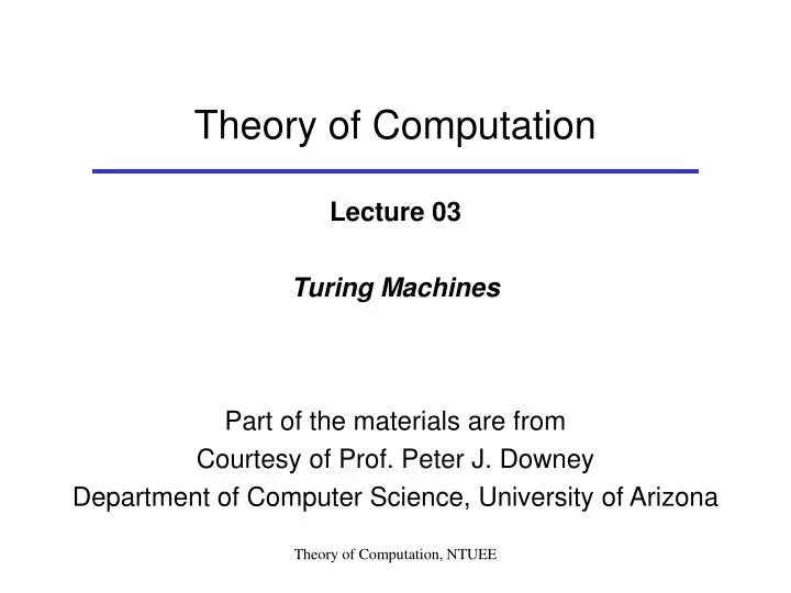
Theory of Computation. Lecture 03 Turing Machines. Part of the materials are from Courtesy of Prof. Peter J. Downey Department of Computer Science, University of Arizona. b. The TM Model. current state. 0 1 2 3 . Unbounded blank tape. .

E N D
Theory of Computation Lecture 03 Turing Machines Part of the materials are from Courtesy of Prof. Peter J. Downey Department of Computer Science, University of Arizona Theory of Computation, NTUEE
b The TM Model current state 0 1 2 3 Unbounded blank tape • Model of ``effectively computable procedure” (including all algorithms) • Primitive as possible (math. simplicity & constructions) • Arbitrary definition choice, but standard • Easy comparison with other models (RAM, p.c.f., etc.) • Finitely describable (just a formatted string) • 1 machine = 1 procedure (no stored program -- different FSA for each TM) • Computes in discrete steps (moves); each step physically trivial • Simple complexity measures (steps=time, cells=space) Fixed # bits R/W head Theory of Computation, NTUEE
b The TM Model 0 1 2 3 • Control unit: FSA with state set Q • Input: character in cell under R/W head • Output: new state & either overstrike character (no head movement) or head movement L or R • Initial state, accept state, reject state: • Tape unit • Finite length string of characters with blanks B to right • Fixed alphabet ( B ); input alphabet • Tape bounded on left Finite- state control Theory of Computation, NTUEE
TM Examples input and R/W head left adjusted at start • TM to scan R over non-blanks to halt over first blank • TM to accept odd parity binary strings 0 B 1 0/0 1/1 0/0 1/1 B B Theory of Computation, NTUEE
TM Definition (1T-DM) • An 8-tuple • Q = finite set of states • = finite tape alphabet; blank B; input alphabet • Transition function • initial state ; halt (accepting/rejecting) states: • Configuration • (1-step) move relation between configurations Note: Below says you can move left from leftmost cell, although you don’t really move left! This convention makes accept, reject the only halt states. Theory of Computation, NTUEE
Acceptance • Move relation (multi-step): • w* is accepted by M • Language accepted by M: • TM-acceptable languages – a class of sets TM • Configuration I is halting: • Nowhere to move: from definition, only2 ways to halt: • A rejecting or accepting configuration: • A configuration for which no move is defined • Initial configuration: • Any halting configuration without is rejecting • Can always arrange that non-accepting, halting configs have • For undefined just add transitions to * * * + Theory of Computation, NTUEE
yes yes Acceptor for L Decider for L w w no Decidable vs. Computably Enumerable • A language L is TM-acceptable iff for some TM M . • M need not, but might, halt rejecting on some strings L • Such a TM is an acceptor or recognizer for L • A language L is decidable (TM-decidable, recursive) iff for some TM M that halts on every input string (whether in L or not). Such a TM is called a decider or algorithm. “procedure” “algorithm” Note: ``yes’’ means enters and halts ``no’’ means enters and halts Theory of Computation, NTUEE
Example • Acceptor for A/ A a/a, X/X b/b,C/C a / A b/X c/C X/X A/A X/X C/C C/C All transitions not shown go to So halts rejecting unless accepting statereached B Theory of Computation, NTUEE
Acceptance (Cont.) • Sequence of configurations is a computation of length (time) t • Computation is in a tight loop iff (a config. repeats) (1) How does a TM accept w? (2) How does a TM reject w? • in a tight loop • a halting & rejecting config • computation never reaches a halting config., and no configuration repeats. This has been called a strange loop NOTE: Can make (1) coincide with halting. Can eliminate (a) in favor of (b). (How?) But there is no algorithm to detect (c ) and eliminate + * * * Theory of Computation, NTUEE
Acceptance (Cont.) • Acceptors and Deciders – summary • M accepts (recognizes) • M decides (is a recognition algorithm for) • rejecting (& halting) • M is called a decision algorithm for S • S is a Computably Enumerable (RE) language if there is some TM that accepts it • S is a Decidable (Recursive) language if there is some TM that decides it • NOTE: every TM accepts some language, but only “special” TMs decide their language * Theory of Computation, NTUEE
TMs As Transducers A TM M computes a function • Whenever f(w) is defined: M started in state with w left-adjusted on its otherwise blank tape enters the accepting halt state with f(w) written left-adjusted on its otherwise blank tape. • Wolog, can assume it halts with the R/W head right adjusted • Whenever f(w) is NOT defined: M started in statewith w left-adjusted on its otherwise blank tape enters a non-accepting halt state or diverges • The function computed by TM M is denoted M(w) • The class of functions computed by TMs is the class of partialcomputable(partial recursive)functions • If a TM halts for all inputs, it implements an algorithm–a total computable (total recursive) function • Confusing traditional terminology: every total computable function is a partial computable function! “partial” doesn’t mean it has to be undefined for some input(!) Theory of Computation, NTUEE
A Look Ahead Characteristic function of a set L: Decidable Computably Enumerable CE sets L Total Computable Functions functions f PCF Theory of Computation, NTUEE
Church’s Thesis (Church-Turing Thesis) The effectively computable functions are those characterized by one of the “standard formalisms” such as the TM. Theory of Computation, NTUEE
TM Examples input and R/W head left adjusted at start TM to copy 0n to the left of ‘1’ While the tape head reads ‘0’, { Change the ‘0’ to ‘1’; Move right; While reading ‘0’, move right. Move right; While not reading blank, move right. Write ‘0’; While reading ‘0’, move left. Move left; While reading ‘0’, move left. Move right; } While not the end of the tape, { Move left; Write ‘0’; } ….. 0 0 0 0 1 FSA ….. 1 0 0 0 0 1 FSA After moving all 0 left, … ….. ….. 1 1 1 1 0 1 0 FSA Theory of Computation, NTUEE
TM Examples input and R/W head left adjusted at start TM that computes 0m+n m n ….. ….. 0 0 0 0 0 0 0 1 FSA copy m m n ….. ….. ….. 0 0 0 0 0 0 0 0 0 0 0 1 FSA Theory of Computation, NTUEE
TM Examples input and R/W head left adjusted at start TM that computes 0mn n m ….. ….. 0 0 1 0 1 0 0 0 Copy once m FSA n n ….. ….. ….. 0 0 0 1 0 1 0 1 0 0 Copy twice m FSA n n n ….. ….. ….. ….. 0 1 0 1 0 1 0 0 1 0 0 0 Copy thrice m FSA n n n ….. ….. ….. ….. 0 1 1 1 0 1 0 0 1 0 0 0 Theory of Computation, NTUEE
TM Extensions: Church’s Thesis • Convenience of having alternate models • Two models of computation are equivalent • whenever a language L is recognized by a machine in one model, there is an algorithm to construct a machine recognizing L in the second, and vice versa • whenever a function f is computed by a machine in one model, there is an algorithm to construct a machine computing f in the second, and vice versa • I.e., Simulation both directions by a “compiling” algorithm Theory of Computation, NTUEE
q TM Extensions: 2-way tape 2-way infinite tape (double-ended tape) TM M • Simulate M by a standard TM Mwith 2 tracks on tape. • Top track for cells at or to right of initial head position (cell 0) • bottom track for cells to left of initial head position • Whenever M crosses over cell 0, Mchanges track under scan • Two tracks simulated by an alphabet ({$}) -4 -3 -2 -1 0 1 2 3 4 q, up Tape symbols (a, b) a,b (a,$) endmark & symbol 0 1 2 3 4 $ -1 -2 -3 -4 In state q, move L from cell 0 shift from state (q, up) to (q, down) In state q, move R from cell 0 shift from state (q, down) to (q, up) Theory of Computation, NTUEE
a b c d e f B . . . A B C D E F G . . . a A TM Extensions: k-tape TM • Tapes simulated by one tape with k tracks & software heads • a in cell iof tape 1 a on track 1 of cell i • a in cell iof tape 1 & head 1 scanning cell on track 1 of cell i • Tape alphabet is head sweeps L to R until store k scanned chars. In states. Sweep R to L & mark changes. Sweep L to R then R to L to move head marks. End cycle scanning cell 0. B B 0 1 2 3 … 0 1 2 3 … b d e f B . . . B C D E G . . . Theory of Computation, NTUEE
k-tape TM (cont.) • Machine uses T+1 cells if makes T steps (& uses a max of T cells on any tape) • Simulating one step of with a max of t cells occupied takes O(t) steps on • Total simulation time for computation of T steps is thus O(n)+O(n+1)+… +O(T ) = where Theory of Computation, NTUEE
a b c d e f B . . . Input tape Read only A B C D E F B . . . Work tape R/W head TM Extensions: Off-line TM • 1 work tape & an additional tape to hold only input • Input tape is read-only; head can move in both directions • Important model in studying spacecomplexity. • Count only the cells dirtied on worktape as “dynamic space” used • There are problems that take only log n extra space beyond space to hold input (e.g.: number of nodes of n-node digraph reachable from a given node) Theory of Computation, NTUEE
TM Extensions: other equivalent models • Multihead TMs – h heads on each of k tapes • Use multiple track idea with head positions by software marks • d-dimensional tape • Grid in 2-dimensions: unbounded N,S,E,W • Can move head +1 in direction N,S,E,W • Use “raster-scan” to linearize the dirtied rectangle of space Theory of Computation, NTUEE
Defn. of Nondeterministic TM (NTM) • 1T-NM: A 8-tuple • Transition function • Configuration • (1-step) move relation between configurations • No reject state • Possible for no next move to be defined for some state: Theory of Computation, NTUEE
Nondeterministic TM • Acceptance: • note the existential quantifier: w is accepted if there is some sequence of “guesses” that drive the initial tape configuration to an accepting configuration • A word w is not accepted iff every possible computation starting with fails to enter an accepting configuration * Theory of Computation, NTUEE
Choice Numbers • Choices for a given state and symbol • For each q and a assign each choice in (q,a) a number • For each machine, there is some largest number of choices for some transition–call it b • Strings over can be interpreted as deterministic directions for which choice to make from each configuration Theory of Computation, NTUEE
Computation Tree Choice sequence Theory of Computation, NTUEE
NTM Equivalent to TM • Theorem 2.3. If L is accepted by an NTM N , there is a DTM D, constructable by algorithm, that accepts L. Proof: Simulate all possible computations on N for all possible choice strings and halt if a sequence of choices is found that leads to an accepting configuration. D has 3 tapes: read-only input, worktape simulating that of N, and an enumeration tape. On the latter, enumerate all choice sequences in lexicographic order Main cycle: generate the next choice seq. c on the enum. Tape. Use this sequence to drive computation of N for a total of |c| steps. If an accepting configuration is reached, D accepts and halts. If the computation halts rejecting, move to the next main cycle after clearing the worktape. Otherwise move to the next main cycle after |c| steps. Iterate the main cycle while an accepting configuration has not been found. If an accepting c exists, D will eventually find it. If none exists, the input will not be accepted. So L(D) = L(N). QED Theory of Computation, NTUEE
A B C D E F B . . . 1-way Read only 1-way Read only 1-way Read only top top a a a b b b c c c d d d e e e f f f B B B . . . . . . . . . . . . $ B C D E F B B B Restricted Models Input tape Output tape • FSA • PD-DM • C-DM (counter machine) 1-way Write only Push-Pop At top only PD contents always of form $1111…11 . . . $ 1 1 1 1 1 B B B Push/Pop At top only Theory of Computation, NTUEE
Results • Old results • 1:-PD-NM = CFL The languages accepted by non-deterministic PDA are exactly the context-free languages • 1:-PD-DM = DCFL CFL There are CFLs that are not among the deterministic CFLs • New results • 1:-2PD-DM = 1T-DM Two pushdown-machines are equivalent to standard TMs • 1:-2C-DM = 1T-DM Two counter machines are equivalent to standard TMs!! Theory of Computation, NTUEE
a b c e f g h j k . . . B B B f g h j k $ $ a b c e i n p u t B B . . . 1:-2PD-DM = 1T-DM • One direction is obvious (2PD-DM is a 2T-DM) • 1T-DM 1:-2PD-DM Proof: B T PD 2 PD 1 Read scanned symbol read PD2 top Write scanned symbol pop PD2; push new on PD2 Move L pop PD1;push PD2 Move R pop PD2; push PD1 Overwrite blanks to right push onto empty PD2 Theory of Computation, NTUEE
Counter Machines • Instead of pushing and popping stacks we will think of counter as a register X and write XX+1, XX-1. We can also test for zero X=0? (sense bottom marker $) • Lemma: 1:-4C-DM = 1T-DM Proof: Show how to simulate onePD by two C. Sort and call ordered symbols PDXY k-ary integer; stack top is low order digit x modk in FSA Theory of Computation, NTUEE
Counter Machines (cont.) • Theorem: 1:-2C-DM = 1:-4C-DM (!) Proof: Show how to simulate 4C with 2C: Theory of Computation, NTUEE