Download
1 / 20
200 likes | 205 Views
This lecture reviews Lecture 9 on F-test problems and provides examples of common cases for model testing, including when coefficients are zero or equal to each other. Steps for model comparison are also discussed.

E N D
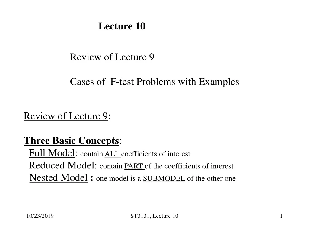
Lecture 10 Review of Lecture 9 Cases of F-test Problems with Examples Review of Lecture 9: Three Basic Concepts: Full Model: contain ALL coefficients of interest Reduced Model: contain PART of the coefficients of interest Nested Model :one model is a SUBMODEL of the other one ST3131, Lecture 10
Common Cases for Model Testing Case 1: ALL NON-intercept coefficients are zero Case 2: SOME of the coefficients are zero Case 3: SOME of the coefficients are EQUAL to each other Case 4: Other specified CONSTRAINTS on coefficients All can be tested using F-test. ST3131, Lecture 10
Steps for Model Comparison : RM H0: The RM is adequate vs FM H1: The FM is adequate Step1: Fit the FM and get SSE (in the ANOVA table) df (in the ANOVA table) R_sq (under the Coefficient Table) Step 2: Fit the RM and get SSE, df, and R_sq. Step 3: Compute F-statistic: Step 4: Conclusion: Reject H0 if F>F(r,df(SSE,F),alpha) Can’t Reject H0 otherwise. ST3131, Lecture 10
Case 1: ALL NON-intercept coefficients are zero Statistical Meaning: ALL predictor variables have no explanatory power the effect of ALL predictor variables are zero. ST3131, Lecture 10
MSR(F)= Mean Square due to REGRESSION for the Full Model MSE(F)=Mean Square due to ERROR for the Full Model =Mean Squared Error for the Full Model The Test can be conducted using an ANOVA (ANalysis Of VAriance) table: ST3131, Lecture 10
Example: the Supervisor Performance Data Analysis of Variance (ANOVA table) Source DF SS MS F P Regression 6 3147.97 524.66 10.50 0.000 Residual Error 23 1149.00 49.96 Total 29 4296.97 Thus, Reject H0, i.e., not all coefficients are zero. ST3131, Lecture 10
The F-test using Multiple Correlation Coefficients R-square The F-test based on ANOVA table is equivalent to the following test based on R-square: ST3131, Lecture 10
Example: the Supervisor Performance Data Results for: P054.txt Regression Analysis: Y versus X1, X2, X3, X4, X5, X6 The regression equation is Y = 10.8 + 0.613 X1 - 0.073 X2 + 0.320 X3 + 0.082 X4 + 0.038 X5 - 0.217 X6 Predictor Coef SE Coef T P Constant 10.79 11.59 0.93 0.362 X1 0.6132 0.1610 3.81 0.001 X2 -0.0731 0.1357 -0.54 0.596 X3 0.3203 0.1685 1.90 0.070 X4 0.0817 0.2215 0.37 0.715 X5 0.0384 0.1470 0.26 0.796 X6 -0.2171 0.1782 -1.22 0.236 S = 7.068 R-Sq = 73.3% R-Sq(adj) = 66.3% F(6,23,.05)=F(6,24,.05)=2.455, F(6,23,.01)=3.80 ST3131, Lecture 10
REMARK: when some of individual coefficients (t-test) are significant, the F-test for testing if all non-intercept coefficients are zero will usually be significant. However, it is possible that none of the non-intercept coefficient t-tests are significant but the F-test is still significant. This implies that the combining explanatory power of the predictor variables is larger than that of any one of the individual predictor variables. ST3131, Lecture 10
Case 2: Some of the Coefficients are zero. If H0 is not rejected and hence is adequate, we should use the Reduced Model. The Principle of Parsimony: always use the ADEQUATE SIMPLER model. Two advantages for using the Reduced Models are 1) Reduced Models are simpler than Full Models 2) The RETAINED predictor variables are emphasized. ST3131, Lecture 10
Example: the Supervisor Performance Data (Continued) Regression Analysis: Y versus X1, X3 The regression equation is Y = 9.87 + 0.644 X1 + 0.211 X3 Predictor Coef SE Coef T P Constant 9.871 7.061 1.40 0.174 X1 0.6435 0.1185 5.43 0.000 X3 0.2112 0.1344 1.57 0.128 S = 6.817 R-Sq = 70.8% R-Sq(adj) = 68.6% Analysis of Variance Source DF SS MS F P Regression 2 3042.3 1521.2 32.74 0.000 Residual Error 27 1254.6 46.5 Total 29 4297.0 SSE(R)=, df(R) =, SSE(F)= df(F)= F=[(SSE(R )-SSE(F))/(df(R )-df(F))]/[SSE(F)/df(F)]= F(4,23,.05)=2.8, Can’t reject H0; the RM is adequate! ST3131, Lecture 10
REMARKS: (1) F-test can be written in terms of the Multiple Correlation Coefficients of the RM and FM. That is, Actually ST3131, Lecture 10
Example: the Supervisor Performance Data (Continued) R_sq(F)= .733, df(F)=23, R_sq(R)=.708, df(R )=27, F=[(.733-.708)/4]/[(1-.733)/23]=.528<2.8=F(4,23,.05), can’t Reject H0 Remark (2): When the RM has only 1 coefficient fewer than the FM, say, beta_j, then r=1, In this case, F-test is equivalent to t-test. ST3131, Lecture 10
Two Remarks about the Coefficients Retaining • The estimates of regression coefficients that do not significantly differ from 0 are often replaced by 0 in the equation. The replacement has two advanatges: a simple model and a smaller prediction variance (the Principle of Parsimony). • A variable or a set of variables may particularly be retained in an equation because of their theoretical importance in a given problem, even though the coefficients are statistically insignificant. For example, the intercept is often retained in the equation even it is not significant in statistical meaning. ST3131, Lecture 10
Case 3: Some Coefficients are equal (I) (II) ST3131, Lecture 10
Example: the Supervisor Performance Data Results for: P054.txt, Regression Analysis: Y versus X1+X3 The regression equation is Y = 9.99 + 0.444 (X1+X3) Predictor Coef SE Coef T P Constant 9.988 7.388 1.35 0.187 X1+X3 0.44439 0.05914 7.51 0.000 S = 7.133 R-Sq = 66.8% R-Sq(adj) = 65.7% Analysis of Variance Source DF SS MS F P Regression 1 2872.4 2872.4 56.46 0.000 Residual Error 28 1424.6 50.9 Total 29 4297.0 SSE (R ) = , df(R )= SSE(F)= df(F)= F={[(SSE(R )-SSE(F)]/[df(R )-df(F)]}/{SSE(F)/df(F)}= =1.10, df=(5,23) F(5,23,.05)=2.49>1.10 So H0 is NOT Rejected. ST3131, Lecture 10
Example: the Supervisor Performance Data (Continued) Regression Analysis: Y versus X1, X3 The regression equation is Y = 9.87 + 0.644 X1 + 0.211 X3 Predictor Coef SE Coef T P Constant 9.871 7.061 1.40 0.174 X1 0.6435 0.1185 5.43 0.000 X3 0.2112 0.1344 1.57 0.128 S = 6.817 R-Sq = 70.8% R-Sq(adj) = 68.6% Analysis of Variance Source DF SS MS F P Regression 2 3042.3 1521.2 32.74 0.000 Residual Error 27 1254.6 46.5 Total 29 4297.0 SSE (R ) = , df(R )= SSE(F)= df(F)= F={[(SSE(R )-SSE(F)]/[df(R )-df(F)]}/{SSE(F)/df(F)}= =3.65, df=(1,27) F(1,27,.05)=4.21>3.65 So H0 is NOT Rejected. ST3131, Lecture 10
Case 4: Other constraints on Coefficients ST3131, Lecture 10
Example: the Supervisor Performance Data (continued) Regression Analysis: Y-X3 versus X1-X3 The regression equation is (Y-X3) = 1.17 + 0.694 (X1-X3) Y=1.17+.694X1+.306 X3 Predictor Coef SE Coef T P Constant 1.167 1.708 0.68 0.500 X1-X3 0.6938 0.1129 6.15 0.000 S = 6.891 R-Sq = 57.4% R-Sq(adj) = 55.9% Analysis of Variance Source DF SS MS F P Regression 1 1794.3 1794.3 37.79 0.000 Residual Error 28 1329.5 47.5 Total 29 3123.9 SSE (R ) = , df(R )= SSE(F)= df(F)= F={[(SSE(R )-SSE(F)]/[df(R )-df(F)]}/{SSE(F)/df(F)}= =1.62, df=(1,27) F(1,27,.05)=4.21>1.62, So H0 is NOT Rejected. ST3131, Lecture 10
After-Class Questions: • What is the difference between F-test and T-test? • If H0 is rejected, does this show that the full model • is better than the reduced model? ST3131, Lecture 10