Download
1 / 34
350 likes | 611 Views
Learning Sequence Motifs Using Expectation Maximization (EM) and Gibbs Sampling. BMI/CS 776 www.biostat.wisc.edu/~craven/776.html Mark Craven craven@biostat.wisc.edu March 2002. Announcements. HW due on Monday reading for next week Chapter 3 of Durbin et al. (already assigned)

E N D
Learning Sequence Motifs Using Expectation Maximization (EM) and Gibbs Sampling BMI/CS 776 www.biostat.wisc.edu/~craven/776.html Mark Craven craven@biostat.wisc.edu March 2002
Announcements • HW due on Monday • reading for next week • Chapter 3 of Durbin et al. (already assigned) • Krogh, An Introduction to HMMs for Biological Sequences • is everyone’s account set up? • did everyone get the Lawrence et al. paper?
Sequence Motifs • what is a sequence motif ? • a sequence pattern of biological significance • examples • protein binding sites in DNA • protein sequences corresponding to common functions or conserved pieces of structure
Motifs and Profile Matrices • given a set of aligned sequences, it is straightforward to construct a profile matrix characterizing a motif of interest shared motif sequence positions 1 2 3 4 5 6 7 8 0.1 0.3 0.1 0.2 0.2 0.4 0.3 0.1 A 0.5 0.2 0.1 0.1 0.6 0.1 0.2 0.7 C G 0.2 0.2 0.6 0.5 0.1 0.2 0.2 0.1 T 0.2 0.3 0.3 0.1 0.2 0.2 0.1 0.3
Motifs and Profile Matrices • how can we construct the profile if the sequences aren’t aligned? • in the typical case we don’t know what the motif looks like • use an Expectation Maximization (EM) algorithm
The EM Approach • EM is a family of algorithms for learning probabilistic models in problems that involve hidden state • in our problem, the hidden state is where the motif starts in each training sequence
The MEME Algorithm • Bailey & Elkan, 1993 • uses EM algorithm to find multiple motifs in a set of sequences • first EM approach to motif discovery: Lawrence & Reilly 1990
Representing Motifs • a motif is assumed to have a fixed width, W • a motif is represented by a matrix of probabilities: represents the probability of character c in column k • example: DNA motif with W=3 1 2 3 A 0.1 0.5 0.2 C 0.4 0.2 0.1 G 0.3 0.1 0.6 T 0.2 0.2 0.1
Representing Motifs • we will also represent the “background” (i.e. outside the motif) probability of each character • represents the probability of character c in the background • example: A 0.26 C 0.24 G 0.23 T 0.27
Basic EM Approach • the element of the matrix represents the probability that the motif starts in position j in sequence I • example: given 4 DNA sequences of length 6, where W=3 1 2 3 4 seq1 0.1 0.1 0.2 0.6 seq2 0.4 0.2 0.1 0.3 seq3 0.3 0.1 0.5 0.1 seq4 0.1 0.5 0.1 0.3
Basic EM Approach given: length parameter W, training set of sequences set initial values for p do re-estimate Z from p (E –step) re-estimate p from Z (M-step) until change in p < e return: p, Z
Basic EM Approach • we’ll need to calculate the probability of a training sequence given a hypothesized starting position: before motif motif after motif is the ith sequence is 1 if motif starts at position j in sequence i is the character at position k in sequence i
G C T G T A G 0 1 2 3 A 0.25 0.1 0.5 0.2 C 0.25 0.4 0.2 0.1 G 0.25 0.3 0.1 0.6 T 0.25 0.2 0.2 0.1 Example
The E-step: Estimating Z • to estimate the starting positions in Z at step t • this comes from Bayes’ rule applied to
The E-step: Estimating Z • assume that it is equally likely that the motif will start in any position
G C T G T A G 0 1 2 3 A 0.25 0.1 0.5 0.2 C 0.25 0.4 0.2 0.1 G 0.25 0.3 0.1 0.6 T 0.25 0.2 0.2 0.1 Example: Estimating Z • then normalize so that ...
The M-step: Estimating p • recall represents the probability of character c in position k ; values for position 0 represent the background pseudo-counts total # of c’s in data set
Example: Estimating p A C A G C A A G G C A G T C A G T C
The EM Algorithm • EM converges to a local maximum in the likelihood of the data given the model: • usually converges in a small number of iterations • sensitive to initial starting point (i.e. values in p)
MEME Enhancements to the Basic EM Approach • MEME builds on the basic EM approach in the following ways: • trying many starting points • not assuming that there is exactly one motif occurrence in every sequence • allowing multiple motifs to be learned • incorporating Dirichlet prior distributions
Starting Points in MEME • for every distinct subsequence of length W in the training set • derive an initial p matrix from this subsequence • run EM for 1 iteration • choose motif model (i.e. p matrix) with highest likelihood • run EM to convergence
Using Subsequences as Starting Points for EM • set values corresponding to letters in the subsequence to X • set other values to (1-X)/(M-1) where M is the length of the alphabet • example: for the subsequence TAT with X=0.5 1 2 3 A 0.17 0.5 0.17 C 0.17 0.17 0.17 G 0.17 0.17 0.17 T 0.5 0.17 0.5
The ZOOPS Model • the approach as we’ve outlined it, assumes that each sequence has exactly one motif occurrence per sequence; this is the OOPS model • the ZOOPS model assumes zero or oneoccurrences per sequence
E-step in the ZOOPS Model • we need to consider another alternative: the ith sequence doesn’t contain the motif • we add another parameter (and its relative) • prior prob that any position in a sequence is the start of a motif • prior prob of a sequence containing a motif
E-step in the ZOOPS Model • here is a random variable that takes on 0 to indicate that the sequence doesn’t contain a motif occurrence
M-step in the ZOOPS Model • update p same as before • update as follows • average of across all sequences, positions
The TCM Model • the TCM (two-component mixture model) assumes zero or more motif occurrences per sequence
Likelihood in the TCM Model • the TCM model treats each length W subsequence independently • to determine the likelihood of such a subsequence: assuming a motif starts there assuming a motif doesn’t start there
E-step in the TCM Model • M-step same as before subsequence isn’t a motif subsequence is a motif
Finding Multiple Motifs • basic idea: discount the likelihood that a new motif starts in a given position if this motif would overlap with a previously learned one • when re-estimating , multiply by • is estimated using values from previous passes of motif finding
Gibbs Sampling • a general procedure for sampling from the joint distribution of a set of random variables by iteratively sampling from for each j • application to motif finding: Lawrence et al. 1993 • can view it as a stochastic analog of EM for this task • less susceptible to local minima than EM
Gibbs Sampling Approach • in the EM approach we maintained a distribution over the possible motif starting points for each sequence • in the Gibbs sampling approach, we’ll maintain a specific starting point for each sequence but we’ll keep resampling these
Gibbs Sampling Approach given: length parameter W, training set of sequences choose random positions for a do pick a sequence estimate p given current motif positions a(update step) (using all sequences but ) sample a new motif position for (sampling step) until convergence return: p, a
Sampling New Motif Positions • for each possible starting position, , compute a weight • randomly select a new starting position according to these weights