• URL : .../publications/courses/ece_8443/lectures/current/lecture_13.ppt

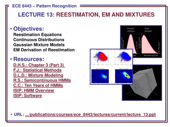
1. LECTURE 13: REESTIMATION, EM AND MIXTURES • Objectives:Reestimation EquationsContinuous DistributionsGaussian Mixture ModelsEM Derivation of Reestimation • Resources:D.H.S.: Chapter 3 (Part 3) F.J.: Statistical MethodsD.L.D.: Mixture ModelingR.S.: Semicontinuous HMMsC.C.: Ten Years of HMMsISIP: HMM OverviewISIP: Software • URL: .../publications/courses/ece_8443/lectures/current/lecture_13.ppt

2. Evaluation and Decoding (Review)

3. Problem No. 3: Learning • Let us derive the learning algorithm heuristically, and then formally derive it using the EM Theorem. • Define a backward probability analogous to i(t): • This represents the probability that we are in state i(t) and will generate the remainder of the target sequence from [t+1,T]. • Define the probability of a transition from i(t-1) to i(t) given the model generated the entire training sequence, vT: • The expected number of transitions from i(t-1) to i(t) at any time is simply the sum of this over T: .

4. Problem No. 3: Learning (Cont.) • The expected number of any transition from i(t) is: • Therefore, a new estimate for the transition probability is: • We can similarly estimate the output probability density function: • The resulting reestimation algorithm is known as the Baum-Welch, or Forward Backward algorithm: • Convergence is very quick, typically within three iterations for complex systems. • Seeding the parameterswith good initial guessesis very important. • The forward backward principle is used in many algorithms.

5. Continuous Probability Density Functions • The discrete HMM incorporates adiscrete probability densityfunction, captured in the matrix B, to describe the probability of outputting a symbol. • Signal measurements, or featurevectors, are continuous-valued N-dimensional vectors. • In order to use our discrete HMM technology, we must vector quantize (VQ) this data – reduce the continuous-valued vectors to discrete values chosen from a set of M codebook vectors. • Initially most HMMs were based on VQ front-ends. However, for the past 20 years, the continuous density model has become widely accepted. • We can use a Gaussian mixture model to represent arbitrary distributions: • Note that this amounts to assigning a mean and covariance matrix for each mixture component. If we use a 39-dimensional feature vector, and 128 mixtures components per state, and thousands of states, we will experience a significant increase in complexity  … 0 1 2 3 6 4 5

6. Continuous Probability Density Functions (Cont.) • It is common to assume that the features are decorrelated and that the covariance matrix can be approximated as a diagonal matrix to reduce complexity. We refer to this as variance-weighting. • Also, note that for a single mixture, the log of the output probability at each state becomes a Mahalanobis distance, which creates a nice connection between HMMs and PCA. In fact, HMMs can be viewed in some ways as a generalization of PCA. • Write the joint probability of the data and the states given the model as: • This can be considered the sum of the product of all densities with all possible state sequences, , and all possible mixture components, K: • and

7. Application of EM • We can write the auxiliary function, Q, as: • The log term has the expected decomposition: • The auxiliary function has three components: • The first term resembles the term we had for discrete distributions. The remaining two terms are new:

8. Reestimation Equations • Maximization of requires differentiation with respect to the parameters of the Gaussian: . This results in the following: • where the intermediate variable, , is computed as: • The mixture coefficients can be reestimated using a similar equation:

9. Summary • Formally introduced a parameter estimation algorithm. • Derived the Baum Welch algorithm using the EM Theorem. • Generalized the output distribution to a continuous distribution using a Gaussian mixture model.