Methods for Dummies General Linear Model

1. Methods for Dummies General Linear Model Samira Kazan &Yuying Liang

2. Part 1 Samira Kazan

3. Overview of SPM Statistical parametric map (SPM) Design matrix Image time-series Kernel Realignment Smoothing General linear model Gaussian field theory Statistical inference Normalisation p <0.05 Template Parameter estimates

4. Question: Is there a change in the BOLD response between seeing famous and not so famous people? Images courtesy of [1], [2]

5. Modeling the measured data Why? Make inferences about effects of interest How? 1) Decompose data into effects and error 2) Form statistic using estimates of effects and error Images courtesy of [1], [2]

6. What is a system? Input Output

7. Images courtesy of [3], [4]

8. Physiology Physics BOLD T2* fMRI • System 2 Neuronal activity Neurovascular coupling Cognition Neuroscience Stimulus • System 1 Images courtesy of [1], [2], [5]

9. System 1 – Cognition / Neuroscience • System 1 Our system of interest Highly non – linear Images courtesy of [3], [6]

10. System 2 – Physics/ Physiology • System 2 Images courtesy of [7-10]

11. System 2 – Physics/ Physiology system 1 is highlynon-linear • System 2 • System 1 system 2 is close to being linear • System 2

12. Linear time invariant (LTI) systems A system is linear if it has the superposition property: ax2(t) + bx2(t)ay2(t) +by2(t) x1(t - T) y1(t - T) x1(t) y1(t) x2(t) y2(t) A fact: If we know the response of a LTI system to some input (i.e. impulse), we can fully characterize the system (i.e. predict what the system will give for any type of input) A system is time invariant if a shift in the input causes a corresponding shift of the output.

13. Linear time invariant (LTI) systems Convolution animation: [11]

14. Measuring HRF

15. Measuring HRF

16. HRF varies substantially across voxels and subjects Variability of HRF Inter-subject variability of HRF Handwerkeret al., 2004, NeuroImage Solution: use multiple basis functions (to be discussed in event-related fMRI) Image courtesy of [12]

17. Variability of HRF

18. Measuring HRF

19. Neuronal activity HRF function = BOLD Signal

20. Neuronal activity HRF function = BOLD Signal

21. =

22. Random Noise + =

23. Linear Drift + =

24. General Linear Model Recap from last week’s lecture Linear regression modelsthe linear relationship between a single dependent variable, Y, and a single independent variable, X, using the equation: Y = β X + c + ε Reflects how much of an effect X has on Y? ε is the error term assumed ~ N(0,σ2)

25. General Linear Model Recap from last week’s lecture Multiple regression is used to determine the effect of a number of independent variables, X1, X2, X3, etc, on a single dependent variable, Y Y = β1X1 + β2X2 +…..+ βLXL + ε reflect the independent contribution of each independent variable, X, to the value of the dependent variable, Y.

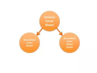
26. General Linear Model General Linear Model is an extension of multiple regression, where we can analyse several dependent, Y, variables in a linear combination: Y1= X11β1+…+X1lβl +…+ X1LβL+ ε1 Yj= Xj1 β1+…+Xjlβl+…+ XjLβL+ εj . . . . . . . . . . . . . . . YJ= XJ1β1 +…+XJlβl+…+ XJLβL+ εJ

27. General Linear Model regressors β1 β2 . . . βL ε1 ε2 . . . εJ Y1 Y2 . . . YJ X11 … X1l … X1L X21… X2l… X2L . . . XJ1 … XJl… XJL = + time points time points time points regressors Y = X *β + ε Design Matrix Observed data Parameters Residuals/Error

28. General Linear Model GLM definition from Huettelet al.: “a class of statistical tests that assume that the experimental data are composed of the linear combination of different model factors, along with uncorrelated noise” General • many simpler statistical procedures such as correlations, t-tests and ANOVAs are subsumed by the GLM Linear • things add up sensibly • linearity refers to the predictors in the model and not necessarily the BOLD signal Model • statistical model

29. General Linear Model and fMRI Famous Not Famous Y= X. β+ ε β1 β2 . . . βp Observed data Y is the BOLD signal at various time points at a single voxel Design matrix Several components which explain the observed BOLD time series for the voxel.Timing info: onset vectors, and duration vectors,HRF.Other regressors, e.g. realignment parameters Parameters Define the contribution of each component of the design matrix to the value of Y Error/residual Difference between the observed data, Y, and that predicted by the model, Xβ.

30. General Linear Model and fMRI Y= X. β+ ε In GLM we need to minimize the sums of squares of difference between predicted values (X β) and observed data (Y), (i.e. the residuals,ε=Y-Xβ) S = Σ(Y-X β)2 S is minimum ∂S/∂β = 0 S β = (XTX)-1 XTY β

31. Beta Weights β is a scaling factor β1 β2 β3 • Larger β Larger height of the predictor (whilst shape remains constant) • Smaller βSmaller height of the predictor (whilst shape remains constant) courtesy of [13]

32. Beta Weights The beta weight is NOT a statistic measure (i.e. NOT correlation) • correlations measure goodness of fit regardless of scale • beta weights are a measure of scale small ß small r small ß large r large ß small r large ß large r courtesy of [13]

33. References (Part 1) • http://en.wikipedia.org/wiki/Magnetic_resonance_imaging • http://www.snl.salk.edu/~anja/links/projectsfMRI1.html • http://www.adhd-brain.com/adhd-cure.html • Dr. Arthur W. Toga, Laboratory of Neuro Imaging at UCLA • https://gifsoup.com/view/4678710/nerve-impulses.html • http://www.mayfieldclinic.com/PE-DBS.htm • http://ak4.picdn.net/shutterstock/videos/344095/preview/stock-footage--d-blood-cells-in-vein.jpg • http://web.campbell.edu/faculty/nemecz/323_lect/proteins/globins.html • http://ej.iop.org/images/0034-4885/76/9/096601/Full/rpp339755f09_online.jpg • http://ej.iop.org/images/0034-4885/76/9/096601/Full/rpp339755f02_online.jpg • http://en.wikipedia.org/wiki/Convolution • Handwerkeret al., 2004, NeuroImage • http://www.fmri4newbies.com/ • http://www.youtube.com/watch?v=vGLd-bUwVXg Acknowledgments: Dr Guillaume Flandin Prof. Geoffrey Aguirre

34. Part 2Yuying Liang

35. Contrasts and Inference • Contrasts: what and why? • T-contrasts • F-contrasts • Example on SPM • Levels of inference

36. First level Analysis = Within Subjects Analysis Time Time Time Time Run 1 Run 1 Run 2 Run 2 First level Subject 1 Subject n Second level group(s)

37. Outline A B C D [1 -1 -1 1] • The Design matrix • What do all the black lines mean? • What do we need to include? • Contrasts • What are they for? • t and F contrasts • How do we do that in SPM12? • Levels of inference

38. ‘X’ in the GLM X = Design Matrix Time (n) Regressors (m)

39. Regressors • A dark-light colour map is used to show the value of each regressor within a specific time point • Black = 0 and illustrates when the regressor is at its smallest value • White = 1 and illustrates when the regressor is at its largest value • Greyrepresents intermediate values • The representation of each regressor column depends upon the type of variable specified )

40. Parameter estimation Objective: estimate parameters to minimize = + Ordinary least squares estimation (OLS) (assuming i.i.d. error): X y

41. Model specification Parameter estimation Hypothesis Statistic Voxel-wise time series analysis Time Time BOLD signal single voxel time series SPM

42. Contrasts: definition and use • To do that contrasts, because: • Research hypotheses are most often based on comparisons between conditions, or between a condition and a baseline

43. Contrasts: definition and use • Contrast vector, named c, allows: • Selection of a specific effect of interest • Statistical test of this effect • Form of a contrast vector: cT = [ 1 0 0 0 ... ] • Meaning: linear combination of the regression coefficients β cTβ = 1 * β1 + 0 * β2 + 0 * β3 + 0 * β4 ...

44. Contrasts and Inference • Contrasts: what and why? • T-contrasts • F-contrasts • Example on SPM • Levels of inference

45. T-contrasts • One-dimensional and directional • egcT = [ 1 0 0 0 ... ] tests β1 > 0, against the null hypothesis H0: β1=0 • Equivalent to a one-tailed / unilateral t-test • Function: • Assess the effect of one parameter (cT = [1 0 0 0]) OR • Compare specific combinations of parameters (cT = [-1 1 0 0])

46. contrast ofestimatedparameters T = varianceestimate T-contrasts • Test statistic: • Signal-to-noise measure: ratio of estimate to standard deviation of estimate

47. T-contrasts: example • Effect of emotional relative to neutral faces • Contrasts between conditions generally use weights that sum up to zero • This reflects the null hypothesis: no differences between conditions [ ½ ½ -1]

48. Contrasts and Inference • Contrasts: what and why? • T-contrasts • F-contrasts • Example on SPM • Levels of inference

49. F-contrasts • Multi-dimensional and non-directional • Tests whether at least one βis different from 0, against the null hypothesis H0: β1=β2=β3=0 • Equivalent to an ANOVA • Function: • Test multiple linear hypotheses, main effects, and interaction • But does NOT tell you which parameter is driving the effect nor the direction of the difference (F-contrast of β1-β2 is the same thing as F-contrast of β2-β1)

50. SSE0 - SSE F = SSE SSE0 SSE F-contrasts • Based on the model comparison approach: Full model explains significantly more variance in the data than the reduced model X0 (H0: True model is X0). • F-statistic: extra-sum-of-squares principle: X0 X1 X0 Full model ? or Reduced model?