Download
1 / 33
330 likes | 437 Views
Words vs. Terms. Words vs. Terms. Information Retrieval cares about “terms” You search for ’em, Google indexes ’em Query: What kind of monkeys live in Costa Rica?. Words vs. Terms. What kind of monkeys live in Costa Rica? words? content words? word stems? word clusters?

E N D
Words vs. Terms 600.465 - Intro to NLP - J. Eisner
Words vs. Terms • Information Retrieval cares about “terms” • You search for ’em, Google indexes ’em • Query: • What kind of monkeys live in Costa Rica? 600.465 - Intro to NLP - J. Eisner
Words vs. Terms • What kind of monkeys live in Costa Rica? • words? • content words? • word stems? • word clusters? • multi-word phrases? • thematic content? (this is a “habitat question”) 600.465 - Intro to NLP - J. Eisner
Finding Phrases (“collocations”) • kick the bucket • directed graph • iambic pentameter • Osama bin Laden • United Nations • real estate • quality control • international best practice • … have their own meanings, translations, etc. 600.465 - Intro to NLP - J. Eisner
Finding Phrases (“collocations”) • Just use common bigrams? • Doesn’t work: • 80871 of the • 58841 in the • 26430 to the • … • 15494 to be • … • 12622 from the • 11428 New York • 10007 he said • Possible correction – just drop function words! 600.465 - Intro to NLP - J. Eisner
Finding Phrases (“collocations”) • Just use common bigrams? • Better correction - filter by tags: A N, N N, N P N … • 11487 New York • 7261 United States • 5412 Los Angeles • 3301 last year • … • 1074 chief executive • 1073 real estate • … 600.465 - Intro to NLP - J. Eisner
Finding Phrases (“collocations”) • Still want to filter out “new companies” • These words occur together reasonably often but only because both are frequent • Do they occur more often than you would expect by chance? • Expect by chance: p(new) p(companies) • Actually observed: p(new companies) • mutual information • binomial significance test [among A N pairs?] = p(new) p(companies | new) 600.465 - Intro to NLP - J. Eisner
data from Manning & Schütze textbook (14 million words of NY Times) N (Pointwise) Mutual Information • p(new companies) = p(new) p(companies) ? • MI = log2p(new companies) / p(new)p(companies)= log2 (8/N) /((15828/N)(4675/N)) = log2 1.55 = 0.63 • MI > 0 if and only if p(co’s | new) > p(co’s) > p(co’s | new) • Here MI is positive but small. Would be larger for stronger collocations. 600.465 - Intro to NLP - J. Eisner
data from Manning & Schütze textbook (14 million words of NY Times) Significance Tests • Sparse data. In fact, suppose we divided all counts by 8: • Would MI change? • No, yet we should be less confident it’s a real collocation. • Extreme case: what happens if 2 novel words next to each other? • So do a significance test! Takes sample size into account. 600.465 - Intro to NLP - J. Eisner
data from Manning & Schütze textbook (14 million words of NY Times) Binomial Significance (“Coin Flips”) • Assume we have 2 coins that were used when generating the text. • Following new, we flip coin A to decide whether companies is next. • Following new, we flip coin B to decide whether companies is next. • We can see that A was flipped 15828 times and got 8 heads. • Probability of this: p8 (1-p)15820 * 15828!/8! 15820! • We can see that B was flipped 14291848 times and got 4667 heads. • Our question: Do the two coins have different weights?(equivalently, are there really two separate coins or just one?) 600.465 - Intro to NLP - J. Eisner
data from Manning & Schütze textbook (14 million words of NY Times) Binomial Significance (“Coin Flips”) • So collocation hypothesis doubles p(data). • We can sort bigrams by the log-likelihood ratio: log pcoll(data)/pnull(data) • i.e., how sure are we that “companies” is more likely after “new”? • Null hypothesis: same coin • assume pnull(co’s | new) = pnull(co’s | new) = pnull(co’s) = 4675/14307676 • pnull(data) = pnull(8 out of 15828)*pnull(4667 out of 14291848) = .00042 • Collocation hypothesis: different coins • assume pcoll(co’s | new) = 8/15828, pcoll(co’s | new) = 4667/14291848 • pcoll(data) = pcoll(8 out of 15828)*pcoll(4667 out of 14291848) = .00081 600.465 - Intro to NLP - J. Eisner
data from Manning & Schütze textbook (14 million words of NY Times) Binomial Significance (“Coin Flips”) • Null hypothesis: same coin • assume pnull(co’s | new) = pnull(co’s | new) = pnull(co’s) = 584/1788460 • pnull(data) = pnull(1 out of 1979)*pnull(583 out of 1786481) = .0056 • Collocation hypothesis: different coins • assume pcoll(co’s | new) = 1/1979, pcoll(co’s | new) = 583/1786481 • pcoll(data) = pcoll(1 out of 1979)*pcoll(583 out of 1786418) = .0061 • Collocation hypothesis still increases p(data), but only slightly now. • If we don’t have much data, 2-coin model can’t be much better at explaining it. • Pointwise mutual information as strong as before, but based on much less data.So it’s now reasonable to believe the null hypothesis that it’s a coincidence. 600.465 - Intro to NLP - J. Eisner
data from Manning & Schütze textbook (14 million words of NY Times) Binomial Significance (“Coin Flips”) • Does this mean that collocation hypothesis is twice as likely? • No, as it’s far less probable a priori! (most bigrams ain’t collocations) • Bayes: p(coll | data) = p(coll) * p(data | coll) / p(data) isn’t twice p(null | data) • Null hypothesis: same coin • assume pnull(co’s | new) = pnull(co’s | new) = pnull(co’s) = 4675/14307676 • pnull(data) = pnull(8 out of 15828)*pnull(4667 out of 14291848) = .00042 • Collocation hypothesis: different coins • assume pcoll(co’s | new) = 8/15828, pcoll(co’s | new) = 4667/14291848 • pcoll(data) = pcoll(8 out of 15828)*pcoll(4667 out of 14291848) = .00081 600.465 - Intro to NLP - J. Eisner
Function vs. Content Words • Might want to eliminate function words, or reduce their influence on a search • Tests for content word: • If it appears rarely? • no: c(beneath) < c(Kennedy) c(aside) « c(oil) in WSJ • If it appears in only a few documents? • better: Kennedy tokens are concentrated in a few docs • This is traditional solution in IR • If its frequency varies a lot among documents? • best: content words come in bursts (when it rains, it pours?) • probability of Kennedy is increased if Kennedy appeared in preceding text – it is a “self-trigger” whereas beneath isn’t 600.465 - Intro to NLP - J. Eisner
abandoned aardvark abacus zymurgy abduct abbot zygote above Latent Semantic Analysis • A trick from Information Retrieval • Each document in corpus is a length-k vector • Or each paragraph, or whatever (0, 3,3,1, 0,7,. . .1, 0) a single document 600.465 - Intro to NLP - J. Eisner
True plot in k dimensions Latent Semantic Analysis • A trick from Information Retrieval • Each document in corpus is a length-k vector • Plot all documents in corpus Reduced-dimensionality plot 600.465 - Intro to NLP - J. Eisner
True plot in k dimensions Latent Semantic Analysis • Reduced plot is a perspective drawing of true plot • It projects true plot onto a few axes • a best choice of axes – shows most variation in the data. • Found by linear algebra: “Singular Value Decomposition” (SVD) Reduced-dimensionality plot 600.465 - Intro to NLP - J. Eisner
True plot in k dimensions theme B theme A word 2 theme B word 3 theme A word 1 Latent Semantic Analysis • SVD plot allows best possible reconstruction of true plot(i.e., can recover 3-D coordinates with minimal distortion) • Ignores variation in the axes that it didn’t pick • Hope that variation’s just noise and we want to ignore it Reduced-dimensionality plot 600.465 - Intro to NLP - J. Eisner
True plot in k dimensions Latent Semantic Analysis • SVD finds a small number of theme vectors • Approximates each doc as linear combination of themes • Coordinates in reduced plot = linear coefficients • How much of theme A in this document? How much of theme B? • Each theme is a collection of words that tend to appear together Reduced-dimensionality plot theme B theme B theme A theme A 600.465 - Intro to NLP - J. Eisner
True plot in k dimensions Latent Semantic Analysis • New coordinates might actually be useful for Info Retrieval • To compare 2 documents, or a query and a document: • Project both into reduced space: do they have themes in common? • Even if they have no words in common! Reduced-dimensionality plot theme B theme B theme A theme A 600.465 - Intro to NLP - J. Eisner
Latent Semantic Analysis • Themes extracted for IR might help sense disambiguation • Each word is like a tiny document: (0,0,0,1,0,0,…) • Express word as a linear combination of themes • Each theme corresponds to a sense? • E.g., “Jordan” has Mideast and Sports themes (plus Advertising theme, alas, which is same sense as Sports) • Word’s sense in a document: which of its themes are strongest in the document? • Groups senses as well as splitting them • One word has several themes and many words have same theme 600.465 - Intro to NLP - J. Eisner
Latent Semantic Analysis • Another perspective (similar to neural networks): terms 1 2 3 4 5 6 7 8 9 matrix of strengths(how strong is eachterm in each document?) Each connection has aweight given by the matrix. 1 2 3 4 5 6 7 documents 600.465 - Intro to NLP - J. Eisner
Latent Semantic Analysis • Which documents is term 5 strong in? terms 1 2 3 4 5 6 7 8 9 docs 2, 5, 6 light up strongest. 1 2 3 4 5 6 7 documents 600.465 - Intro to NLP - J. Eisner
Latent Semantic Analysis • Which documents are terms 5 and 8 strong in? terms 1 2 3 4 5 6 7 8 9 This answers a query consisting of terms 5 and 8! really just matrix multiplication:term vector (query) x strength matrix = doc vector . 1 2 3 4 5 6 7 documents 600.465 - Intro to NLP - J. Eisner
gives doc 5’s coordinates! Latent Semantic Analysis • Conversely, what terms are strong in document 5? terms 1 2 3 4 5 6 7 8 9 1 2 3 4 5 6 7 documents 600.465 - Intro to NLP - J. Eisner
Latent Semantic Analysis • SVD approximates by smaller 3-layer network • Forces sparse data through a bottleneck, smoothing it terms terms 1 2 3 4 5 6 7 8 9 1 2 3 4 5 6 7 8 9 themes 1 2 3 4 5 6 7 1 2 3 4 5 6 7 documents documents 600.465 - Intro to NLP - J. Eisner
Latent Semantic Analysis • I.e., smooth sparse data by matrix approx: M A B • A encodes camera angle, B gives each doc’s new coords terms terms 1 2 3 4 5 6 7 8 9 1 2 3 4 5 6 7 8 9 A matrix M themes B 1 2 3 4 5 6 7 1 2 3 4 5 6 7 documents documents 600.465 - Intro to NLP - J. Eisner
Latent Semantic Analysis Completely symmetric! Regard A, B as projecting terms and docs into a low-dimensional “theme space” where their similarity can be judged. terms terms 1 2 3 4 5 6 7 8 9 1 2 3 4 5 6 7 8 9 A matrix M themes B 1 2 3 4 5 6 7 1 2 3 4 5 6 7 documents documents 600.465 - Intro to NLP - J. Eisner
Latent Semantic Analysis • Completely symmetric. Regard A, B as projecting terms and docs into a low-dimensional “theme space” where their similarity can be judged. • Cluster documents (helps sparsity problem!) • Cluster words • Compare a word with a doc • Identify a word’s themes with its senses • sense disambiguation by looking at document’s senses • Identify a document’s themes with its topics • topic categorization 600.465 - Intro to NLP - J. Eisner
If you’ve seen SVD before … • SVD actually decomposes M = A D B’ exactly • A = camera angle (orthonormal); D diagonal; B’ orthonormal terms terms 1 2 3 4 5 6 7 8 9 1 2 3 4 5 6 7 8 9 A matrix M D B’ 1 2 3 4 5 6 7 1 2 3 4 5 6 7 documents documents 600.465 - Intro to NLP - J. Eisner
If you’ve seen SVD before … • Keep only the largest j < k diagonal elements of D • This gives best possible approximation to M using only j blue units terms terms 1 2 3 4 5 6 7 8 9 1 2 3 4 5 6 7 8 9 A matrix M D B’ 1 2 3 4 5 6 7 1 2 3 4 5 6 7 documents documents 600.465 - Intro to NLP - J. Eisner
If you’ve seen SVD before … • Keep only the largest j < k diagonal elements of D • This gives best possible approximation to M using only j blue units terms terms 1 2 3 4 5 6 7 8 9 1 2 3 4 5 6 7 8 9 A matrix M D B’ 1 2 3 4 5 6 7 1 2 3 4 5 6 7 documents documents 600.465 - Intro to NLP - J. Eisner
If you’ve seen SVD before … • To simplify picture, can write M A (DB’) = AB terms terms 1 2 3 4 5 6 7 8 9 1 2 3 4 5 6 7 8 9 A matrix M B = DB’ 1 2 3 4 5 6 7 1 2 3 4 5 6 7 documents documents • How should you pick j (number of blue units)? • Just like picking number of clusters: • How well does system work with each j (on held-out data)? 600.465 - Intro to NLP - J. Eisner