Download
1 / 20
200 likes | 317 Views
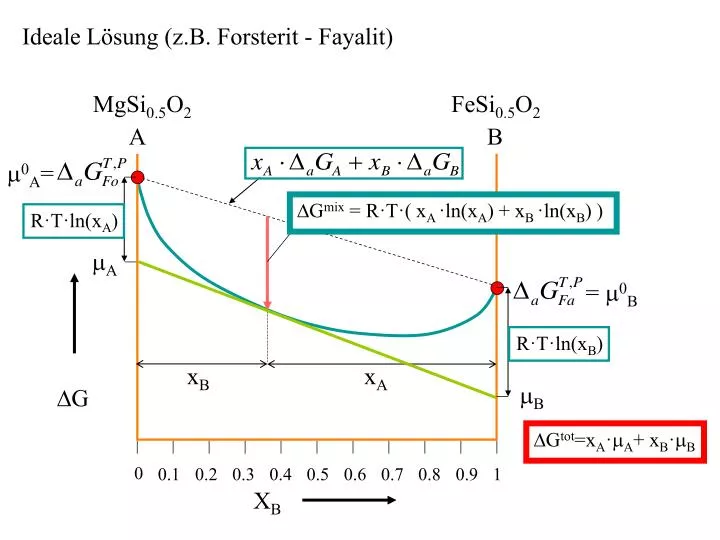
Ideale Lösung (z.B. Forsterit - Fayalit). MgSi 0.5 O 2. FeSi 0.5 O 2. A. B. 0 A =. ∆G mix = R·T·( x A ·ln(x A ) + x B ·ln(x B ) ). R·T·ln(x A ). A. = 0 B. R·T·ln(x B ). x B. x A. B. ∆G. ∆G tot =x A · A + x B · B. 0. 0.1. 0.2. 0.3. 0.4. 0.5. 0.6. 0.7. 0.8.

E N D
Ideale Lösung (z.B. Forsterit - Fayalit) MgSi0.5O2 FeSi0.5O2 A B 0A= ∆Gmix = R·T·( xA ·ln(xA) + xB ·ln(xB) ) R·T·ln(xA) A = 0B R·T·ln(xB) xB xA B ∆G ∆Gtot=xA·A+ xB·B 0 0.1 0.2 0.3 0.4 0.5 0.6 0.7 0.8 0.9 1 XB
MgSi0.5O2 0Fo' = 2·0Fo Mg2SiO4 ∆Gmix = 2· ( xFo·(0Fo+ R·T· ln(xFo)) + xFa·(0Fa+ R·T· ln(xFa)) ) 0Fa' = 2·0Fa Fe2SiO4 0Fo ∆Gmix = ( xFo·(0Fo+ R·T· ln(xFo)) + xFa·(0Fa+ R·T· ln(xFa)) ) 0Fa FeSi0.5O2 ∆G 0 0.1 0.2 0.3 0.4 0.5 0.6 0.7 0.8 0.9 1 XB
∆Gmix = 2· ( xFo·(0Fo+ R·T· ln(xFo)) + xFa·(0Fa+ R·T· ln(xFa)) ) ∆Gmix = xFo·2·(0Fo+ R·T· ln(xFo)) + xFa·2·(0Fa+ R·T· ln(xFa)) ) ∆Gmix = ( xFo·2·0Fo+ xFo·2· R·T· ln(xFo) + xFa·2·0Fa+ xFa·2· R·T·ln(xFa) ) ∆Gmix = ( xFo·0Fo'+ xFo·2· R·T· ln(xFo) + xFa·0Fa'+ xFa·2· R·T· ln(xFa) ) ∆Gmix = ( xFo·0Fo'+ xFo· R·T· ln(xFo2) + xFa·0Fa'+ xFa· R·T· ln(xFa2) ) Def: aFo = xFo2 ∆Gmix = ( xF'·0Fo'+ xFo· R·T· ln(aFo) + xFa·0Fa'+ xFa· R·T· ln(aFa) )
∆Gmix = ( xF'·0Fo'+ xFo· R·T· ln(aFo) + xFa·0Fa'+ xFa· R·T· ln(aFa) ) Fo (Mg2SiO4) - Fa (Fe2SiO4) Wahrscheinlichkeit, dass bei Statistischer Verteilung der Ionen, in einer willkürlich ausgewählten Elementarzelle (X2SiO4) die Konfiguration (Spezies) Mg2SiO4 auftritt: xMg·xMg = xMg2 = aFo Fo = Fo0+RT·ln(xMg2)
∆Gmix = ∑( xi·(0i + R·T· ln(ai) ) Zusammenfassung: Die Aktivität (a) einer Phase ist gleich der Wahrscheinlichkeit ihres Auftretens in der Lösung. Im idealen Fall ist dies gleich ihrer Konzentration. Die "ideale Aktivität" oder Konfigurationelle Aktivität einer Phase ist die statistische Wahrscheinlichkeit ihres Auftretens. Abweichungen von dieser Wahrscheinlichkeit werden als nicht-ideal bezeichnet. ideale Lösung: ai = xi auch ideale Lösung: ai = xin (spezialfall, da nur auf einem Gitterplatz gemischt)
∆Gmix = ∑( xi·(0i + R·T·ln(ai) ) Ein einfaches Beispiel: Orthopyroxene Orthopyroxene haben zwei verschiedene oktaedrische Gitterplätze: M1 und M2 Enstatit (Mg2SiO3) Ferrosilit (Fe2SiO3) Mögliche Konfigurationen in einem Mischkristall sind: (MgMg)SiO3 - (MgFe)SiO3 - (FeMg)SiO3 - (FeFe)SiO3 Beispiel xEn=0.5, xFs=0.5: Rein statistisch erwarten wir: aEn = xEn2 = 0.25 Extremfälle: (FeFe)SiO3 und (MgMg)SiO3 sind viel stabiler als (MgFe)SiO3 und (FeMg)SiO3 aEn = 0.5 (MgFe)SiO3 und (FeMg)SiO3 sind viel stabiler als (FeFe)SiO3 und (MgMg)SiO3 aEn = 0 (FeMg)SiO3 ist völlig unstabil aEn = 0.33 etc.
Al Si Si Al Ca Na Ca Si Al Si Ein etwas komplizierteres Beispiel: Albit (NaAlSi3O8) Anorthit (CaAl2Si2O8) Na Gitterplätze A1, A2, ...: Na, Ca Gitterplätze T1, T2, ...: Si, Al Gitterplätze O1, O2, ...: O
identisch zu idealer Lösung aAb = xAb aAn = xAn Modell 2: (Molecular Model) Gitterplätze A alle äquivalent nur ein T1 Gitterplatz für Si und Al zur verfügung Gekoppelter Ersatz: NaASiT1 CaAAlT1 Albit (NaAlSi3O8) Anorthit (CaAl2Si2O8)
Ab: xNaA =1, xSiT1 = 1/2, xAlT1 = 1/2 An: xCaA =1, xAlT1 = 1 aAb = xNaA ·2xSiT1 ·2xAlT1 aAn = xCaA ·xAlT1 ·xAlT1 xNaA = xAb xCaA = xAn xSiT1 = xAb/2 xAlT1 = xAb/2 + xAn aAb = xAb·(1-xAn2) aAn = (1/4)·xAn·(1+xAn)2 Modell 1: (Al-avoidance with no local charge balance) Gitterplätze A alle äquivalent Gitterplatz T1: Si, Al, alle anderen: Si Albit (NaAlSi3O8) Anorthit (CaAl2Si2O8)
aAb = xAb·(1-xAn2) aAn = (1/4) ·xAn·(1+xAn)2 ∆Gmix = R·T·( xAb·ln(aAb) + xAn·ln(aAn) )
aAb = xAb aAb = xAb·(1-xAn2) aAn = xAn aAn = (1/4) ·xAn·(1+xAn)2 ∆Gmix = R·T·( xAb·ln(aAb) + xAn·ln(aAn) )
aAb = xAb aAb = xAb·(1-xAn2) aAn = xAn aAn = (1/4) ·xAn·(1+xAn)2 ∆Gmix = R·T·( xAb·ln(aAb) + xAn·ln(aAn) ) "real" (gefittet)
aAb = xAb aAb = xAb·(1-xAn2) aAn = xAn aAn = (1/4) ·xAn·(1+xAn)2 Differenz: "real" - Modell 1 ∆Gmix = R·T·( xAb·ln(aAb) + xAn·ln(aAn) ) "real" (gefittet)
aAb = xAb·(1-xAn2) aAn = (1/4) ·xAn·(1+xAn)2 Exzess-Funktion: Polynom ∆Gex = W112·xAb2·xAn + W122·xAb·xAn2 ∆Gmix = R·T·( xAb·ln(aAb') + xAn·ln(aAn') ) ∆Gmix = R·T·( xAb·ln(aAb) + xAn·ln(aAn) ) + ∆Gex Differenz: "real" - Modell 1 ∆Gmix = R·T·( xAb·ln(aAb) + xAn·ln(aAn) )
Nicht-ideale Lösungen: Die Exzess-Funktion ∆Gmix = R·T·∑( xi·(0i + ln(ai) ) ∆Gmix = R·T·∑( xi·(0i + ln(xi) ) + ∆GEx Definition des Aktivitätskoeffizeinten: ai = xi · gi ∆Gmix = R·T·∑( xi·(0i + ln(xi) + ln(gi) ) ∆GEx = R·T·∑( xi·ln(gi) ) weniger strenge Definition ∆Gmix = R·T·∑( xi·(0i + ln(ai) ) ∆Gmix = R·T·∑( xi·(0i + ln(xi) + ln(gconfi) ) + ∆GEx Definition des Aktivitätskoeffizeinten: ai = xi · gconfi · gExi ∆Gmix = R·T·∑( xi·(0i + ln(xi) + ln(gconfi) + ln(gExi) ) ∆GEx = R·T·∑( xi·ln(gExi) )
WAB = Margules-Parameter Andere Schreibweise: Nicht-ideale Lösungen: Die Exzess-Funktion ∆GEx = polynom 2. Grads ∆GEx = a·xB2 + b·xB + c Randbedingungen: xB = 0 ∆GEx = 0 xB = 1 ∆GEx = 0 (da xA = 0) c = 0, b = -a ∆GEx = a·xB2 - a·xB = a·xB·(1-xB) ∆GEx = WAB·xA·xB (symmetrische Lösung)
Andere Schreibweise (da (xA+xB)=1): WAAB, WABB = Margules-Parameter Nicht-ideale Lösungen: Die Exzess-Funktion ∆GEx = polynom 3. Grads ∆GEx = a·xB3 + b·xB2 + c·xB + d Randbedingungen: xB = 0 ∆GEx = 0 xB = 1 ∆GEx = 0 (da xA = 0) d = 0, c = -a-b ∆GEx = a·xB3 - b·xB2 -(a+b)·xB ∆GEx = WAAB·xA2·xB + WABB·xA·xB2 (reguläre Lösung)
Nicht-ideale Lösungen: Beispiel ∆GEx = WAAB·xA2·xB + WABB·xA·xB2 WAAB = WHAAB - T·WSAAB + (P-1)· WVAAB WABB = WHABB - T·WSABB + (P-1)· WVABB