Download

1 / 26
260 likes | 275 Views
Nuovi algoritmi di b tagging. Alessia Tricomi Università and INFN Catania. TISB – Firenze 15-16 Gennaio 2003. Alcune considerazioni sullo stato dei tools. Cosa c’è di pronto Track counting e Probabilistico a “la ALEPH” già inseriti da Gabriele nel suo framework Nuovi algoritmi “stand alone”

E N D
Nuovi algoritmi di b tagging Alessia Tricomi Università and INFN Catania TISB – Firenze 15-16 Gennaio 2003
Alcune considerazioni sullo stato dei tools • Cosa c’è di pronto • Track counting e Probabilistico a “la ALEPH” già inseriti da Gabriele nel suo framework • Nuovi algoritmi “stand alone” • Likelihood ratio • Implementazione • Primi risultati mostrati durante la CMS Week di Dicembre • Leptonico • Idea • Implementazione • Problemi • Cosa serve • C’è un framework sviluppato da Gabriele che integra già alcuni algoritmi (vedi presentazione di Gabriele) in cui però bisogna integrare i nuovi algoritmi ed eventualmente renderlo più flessibile • Occorre un pacchetto semplice e user friendly per la calibrazione degli algoritmi probabilistici
Cosa vi mostro ora? • Un riassunto del Likelihood Ratio con i primi risultati • Uno schema del btagging con leptoni • Una discussione sui problemi Rimandiamo la discussione su cosa serve e come farlo alla fine delle presentazioni…
Linearised track Jet Helix Pa PV do The main idea • b-jet tagging made exploiting long lifetime of b: • the algorithm relies on tracks with large impact parameter • Both transverse and 3D IP have been used • A probabilistic approach is used • Sign is positive if track appears to originate in front of PV • Negative if it appears to originate from behind Significance of IP is defined as the ratio of the signed IP to its total error: sign x |d0|/s(d0) (take better in account experimental resolutions)
Probabilistic algorithms • Tracksfrom b hadron decays have usually LARGE and POSITIVE IP • Tracks coming from the PV and badly reconstructed tracks have a 50% chance to be assigned a negative significance • Tracks with negativeIP dused however to measure the intrinsic resolution(due to limitedresolution on track reconstruction, primary vertex finding, b-jet reconstruction) • Confidence level that a track with IP significance SD originates from the primary vertex given by: • By construction the C.L. is flat for tracks coming from primary vertex while is peaked at small values for tracks coming from displaced vertices
Probabilistic algorithms • Starting from the C.L. the probability that a set of tracks is coming from the PV can be evaluated • In the Likelihood ratio method however both bkg and signal information are used: • b-jet to bkg-jet ratio: builds a global likelihood ratio based on the distributions of SD expected for b-jets and bkg (gluon or uds) jets. The sum over all selected tracks of lg(ratio) provides discrimination between jets wich contain long-lived particles and those which do not.
Likelihood ratio: the method Main step of the method: • For each track i in a jet the significance Si is evaluated • The ratio of the significance probability distribution functions for b and u-jets is computed: ri= fb(Si)/ fu(Si) • A jet weight is constructed from the sum of logarithms of the ratio: W=Slog ri • By keeping jets above some value of W, the efficiency for different jet samples can be obtained • The rejection will have to be optimised for each specific bkg under study • Several track quality cuts applied
Samples & Track Selection • Monte Carlo samples: • bb, cc and uu events • Jet Transverse Energies: 50, 100 and 200 GeV • |h| intervals considered: • |h| < 0.7 • 0.7 < |h| < 1.4 • 1.4 < |h| < 2.0 • 2.0 < |h| < 2.4 • Track selection (ORCA_6_1_1): • Forward Kalman Filter used for track reconstruction • Tracks with p > 1 GeV • Tracks inside the jet within a DR<0.4 cone size • At least 8 hits per track • At least 3 hits in the pixel • To reject g conversions, L and KS decays, Transverse IP < 2 mm
Track quality classes • IP measurements depend on momentum and number of hits in the different kind of detectors 8 Quality track classes defined: Nhit 8 • h0.7 • p < 5 • p > 5 • 0.7 < h 1.4 • p < 10 • p > 10 • 0.7 < h 1.4 • p < 15 • p > 15 • 0.7 < h 1.4 • p < 20 • p > 20
First step: resolution function calibrations • Resolution function dominated by Gaussian term+exponential terms (effects not taken into account in the error estimate, secondary interactions with the material and lifetime) bb ET=100 GeV h0.7 p < 5 p > 5 0.7 < h 1.4 p < 10 p > 10
First step: resolution function calibrations bb ET=100 GeV 1.4 < h 2.0 p < 15 p > 15 2.0 < h 2.4 p < 20 p > 20
First step: resolution function calibrations cc ET=100 GeV h0.7 p < 5 p > 5 0.7 < h 1.4 p < 10 p > 10
First step: resolution function calibrations cc ET=100 GeV 1.4 < h 2.0 p < 15 p > 15 2.0 < h 2.4 p < 20 p > 20
First step: resolution function calibrations uds ET=100 GeV h0.7 p < 5 p > 5 0.7 < h 1.4 p < 10 p > 10
First step: resolution function calibrations uds ET=100 GeV 1.4 < h 2.0 p < 15 p > 15 2.0 < h 2.4 p < 20 p > 20
Likelihood ratio: distribuzione Wjet ORCA 6.1.1
Likelihood ratio: performances Preliminary: calibration to optimize Mistag = 5% eb70%,eb65%* Mistag = 10% eb80%,eb72%* Mistag = 20% eb85%,eb78%* * DAQTDR
Likelihood ratio: performances 1.4 < h 2.4 ex
Likelihood ratio: performances |h| 1.4 ex
Likelihood ratio: performances 1.4 < |h| 2.4 ex
Likelihood ratio: performances |h| 1.4 ex
Likelihood ratio: performances 1.4 < |h| 2.4 ex
Conclusions • Performances seem interesting • Results are very preliminary • 3D performances still need to be studied • More statistics needed for calibration • Staged scenario need to be studied • New ORCA should be used • Rejection need to be optimized for each specific bkg under study
b tagging con i leptoni: idea • La presenza di leptoni soft provenienti dai decadimenti semileptonici dei mesoni B può essere utilizzata per taggare i jet di b • L’efficienza del soft lepton tagging è limitata dalla frazione di decadimenti semileptonici dei B ( 17%) • Leptoni di segnale in b-jets: • Decadimenti diretti: b l • Decadimenti in cascata: b cl • Decadimenti leptonici della J/y : b J/yl • Decadimenti di adroni b in t e poi in l: b tl • Electroni di fondo: • Conversioni g • Decadimenti Dalitz di p0 • Decadimenti semileptonici in cascate di adroni • Muoni di fondo: • Muoni da decadimenti di K e p • Particelle misidentified in jet contenenti muoni reali • (muoni di basso pT ) particelle estrapolate alle camere per muoni con depositi di energia compatibili con muoni
b tagging con i leptoni: realizzazione • Primo approccio: per ora solo con i muoni • Ricostruire i jet, guardare alle tracce del jet, ricostruire i muoni di L3 e fare un match traccia-muone • Secondo approccio: • Ricostruire tutti i muoni di L2 • Per i muoni di L2 all’interno del cono del jet ricostruire i muoni di L3 in questo modo si ricostruiscono solo le tracce compatibili con i muoni • Ma… PROBLEMA!!! • La ricostruzione dei muoni e l’uso della libreria bTauJetTools sembrano incompatibili! Basta includere questa libreria perché la RecCollection dei muoni risulti vuota! • Il prossimo step: • innanzitutto occorre risolvere il problema muoni-bTauJet • Fatto questo la realizzazione dell’algoritmo dovrebbe essere abbastanza rapida. Uno schema di algoritmo è già pronto
Conclusioni Ne parliamo dopo…