Download

1 / 46
460 likes | 539 Views
Impacts on Suply Arising from Changes In Supply Determinants. SUPPLY SHIFTS. Percentage change in Q s. Price elasticity of supply. =. Percentage change in P. Price Elasticity of Supply. 0. Price elasticity of supply measures how much Q s responds to a change in P. P. S.

E N D
Impacts on Suply Arising from Changes In Supply Determinants
Percentage change in Qs Price elasticity of supply = Percentage change in P Price Elasticity of Supply 0 • Price elasticity of supply measures how much Qs responds to a change in P.
P S Percentage change in Qs Price elasticity of supply = P2 Percentage change in P P1 Q Q1 Q2 16% = 2.0 8% Price Elasticity of Supply 0 Price elasticity of supply equals Example: P rises by 8% Q rises by 16%
% change in Q Price elasticity of supply = = % change in P P S P2 Q “Perfectly inelastic” (one extreme) 0 0% = 0 10% S curve: vertical Sellers’ price sensitivity: P1 0 Elasticity: Q1 0 P rises by 10% Q changes by 0%
% change in Q Price elasticity of supply = = % change in P P S P2 Q Q2 “Inelastic” 0 < 10% < 1 10% S curve: relatively steep Sellers’ price sensitivity: P1 relatively low Elasticity: Q1 < 1 Q rises less than 10% P rises by 10%
% change in Q Price elasticity of supply = = % change in P P S P2 Q Q2 “Unit elastic” 0 10% = 1 10% S curve: intermediate slope Sellers’ price sensitivity: P1 intermediate Elasticity: Q1 = 1 Q rises by 10% P rises by 10%
% change in Q Price elasticity of supply = = % change in P P S P2 Q Q2 “Elastic” 0 > 10% > 1 10% S curve: relatively flat Sellers’ price sensitivity: P1 relatively high Elasticity: Q1 > 1 Q rises more than 10% P rises by 10%
% change in Q Price elasticity of supply = = % change in P P S Q Q1 Q2 “Perfectly elastic”(the other extreme) 0 any % = infinity 0% S curve: horizontal P1 P2 = Sellers’ price sensitivity: extreme Elasticity: infinity Q changes by any % P changes by 0%
P S D1 D2 B P2 P1 A Q Q1 Q2 When supply is inelastic, an increase in demand has a bigger impact on price than on quantity. inelastic supply: 13
P D1 D2 S B P2 A P1 Q Q2 Q1 When supply is elastic, an increase in demand has a bigger impact on quantity than on price. elastic supply 14
P S $15 12 4 $3 Q 100 200 500 525 How the Price Elasticity of Supply Can Vary 0 Supply often becomes less elastic as Q rises, due to capacity limits. elasticity < 1 elasticity > 1
D S S’ P1 P3 Q1 Q3 Q2 Changes In Market Equilibrium • Raw material prices fall • S shifts to S’ • Surplus @ P1 of Q1, Q2 • Equilibrium @ P3, Q3 P Q
D D’ S S’ P2 P1 Q1 Q2 Changes In Market Equilibrium • Income Increases & raw material prices fall • The increase in D is greater than the increase in S • Equilibrium price and quantity increase to P2, Q2 P Q
Prices fell until a new equilibrium was reached at $0.26 and a quantity of 5,300 million dozen S1970 S1998 $0.61 $0.26 D1970 D1998 5,300 5,500 Market for Eggs P (1970 dollars per dozen) Q (million dozens)
S1995 Prices rose until a new equilibrium was reached at $4,573 and a quantity of 12.3 million students $4,248 S1970 $2,530 D1995 D1970 8.6 14.9 Market for a College Education P (annual cost in 1970 dollars) Q (millions of students enrolled))
Price S1900 S1950 S1998 Long-Run Path of Price and Consumption D1900 D1950 D1998 Quantity Changes In Market Equilibrium
The Market for Wheat • 1981 Supply Curve for Wheat • QS = 1,800 + 240P • 1981 Demand Curve for Wheat • QD = 3,550 - 266P
The Market for Wheat • Equilibrium: Q S = Q D
Elasticities of Supply and Demand The Market for Wheat
Elasticities of Supply and Demand The Market for Wheat • Assume the price of wheat is $4.00/bushel
Applications of Supply and Demand • Interference with the Price Mechanism: • the effect of a price ceiling • the effect of a price floor • the effect of a subsidy • the incidence of taxes
KEBIJAKAN PEMERINTAH DALAM MENSTABILKAN HARGA • KEBIJAKAN HARGA MAKSIMUM (Price Ceilings) • PEMERINTAH MENETAPKAN HARGA MAKSIMUM TERHADAP SUATU PRODUK, SEHINGGA MASYRAKAT DAPAT MEMPEROLEH DENGAN HARGA RENDAH • KELEMAHANNYA: • Terjadi kelebihan permintaan, timbul pasar gelap, karena pembeli banyak, penjual dapat menjual secara sembunyi-sembunyi • Untuk mengatasi pasar gelap: • - Menegakkan hukuman dan denda secara tegas • - Melakukan penjatahan
P S Price ceiling $500 shortage D Q 400 250 How Price Ceilings Affect Market Outcomes The eq’m price ($800) is above the ceiling and therefore illegal. The ceiling is a binding constrainton the price, and causes a shortage. $800
P S Price ceiling $1000 $800 D Q 300 How Price Ceilings Affect Market Outcomes A price ceiling above the eq’m price is not binding – it has no effect on the market outcome.
P S Price ceiling $500 shortage D Q How Price Ceilings Affect Market Outcomes In the long run, supply and demand are more price-elastic. So, the shortage is larger. $800 450 150
KEBIJAKAN PEMERINTAH DALAM MENSTABILKAN HARGA • KEBIJAKAN HARGA MINIMUM (Price Floors ) • PEMERINTAH MENETAPKAN HARGA MINUMUM ATAU KEBIJAKAN HARGA TERENDAH • contoh: Harga Gabah • Pemerintah menetapkan harga beli gabah minimum untuk melindungi petani • KELEMAHANNYA: • Terjadi kelebihan penawaran, untuk ini pemerintah harus membeli gabah atau mengekspor supaya stok gabah di pasar tidak banyak.
labor surplus W S Price floor $5 $4 D L 400 550 How Price Floors Affect Market Outcomes The eq’m wage ($4) is below the floor and therefore illegal. The floor is a binding constrainton the wage, and causes a surplus (i.e., unemployment).
W S Price floor $3 $4 D L 500 How Price Floors Affect Market Outcomes A price floor below the eq’m price is not binding – it has no effect on the market outcome.
unemp-loyment W S Min. wage $5 $4 D L 400 550 The Minimum Wage Min wage laws do not affect highly skilled workers. They do affect teen workers. Studies: A 10% increase in the min wage raises teen unemployment by 1-3%.
Kelebihan Penawaran 5 Price floor dan Excess Suypply
KEBIJAKAN PEMERINTAH DALAM MENSTABILKAN HARGA • KEBIJAKAN SUBSIDI • PEMERINTAH MEMBERIKAN SUBSIDI, SUPAYA PENDAPATAN PRODUSEN TIDAK MERUGI • contoh: Harga Produk Pertanian • Kalau diserahkan pada mekanisme pasar, Harga yang diterima Petani tidak mencukupi untuk mendapatkan pendapatan layak • Pemerintah memberi subsidi terhadap produk yang dihasilkan, akibatnya semua petani berupaya meningkatkan produksinya. Kurve penawaran berubah • Harga setelah subsidi sebesar P2 , Kenaikan produksi menjadi Q1 • Pendapatan petani menjadi 0Q1E1P1, subsidi pemerintah P1E1E2P2 • Pendapatan petani dengan subsidi menjadi 0Q1E2P2
KEBIJAKAN PEMERINTAH DALAM MENSTABILKAN HARGA • KEBIJAKAN PAJAK • UNTUK MELINDUNGI PRODUK DALAM NEGERI,PEMERINTAH MENGENAKAN PAJAK TERHADAP PRODUK IMPOR • DAMPAK KENAIKAN TERGANTUNG PADA: • - ELASTISITAS PERMINTAAN • - ELASTISITAS PENAWARAN