Download
1 / 51
560 likes | 1.09k Views
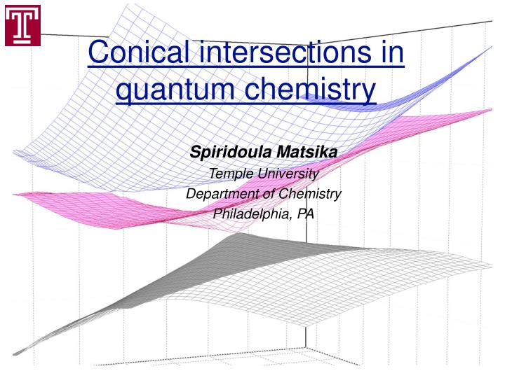
Conical intersections in quantum chemistry. Spiridoula Matsika Temple University Department of Chemistry Philadelphia, PA. Nonadiabatic events in chemistry and biology. Molecular Hamiltonian. e 2 /r ij. i. j. Z e 2 /r i . Z e 2 /r j . Z Z e 2 /R . . .

E N D
Conical intersections in quantum chemistry Spiridoula Matsika Temple University Department of Chemistry Philadelphia, PA
Molecular Hamiltonian e2/rij i j Ze2/ri Ze2/rj ZZe2/R
The Born-Oppenheimer (adiabatic) approximation Separate the problem into an electronic and a nuclear part Nuclear Electronic
When electronic states approach each other, more than one of them should be included in the expansion Born-Huang expansion If the expansion is not truncated the wavefunction is exact since the set Ie is complete Derivative coupling
Two-state conical intersections Two adiabatic potential energy surfaces cross (E=0).The interstate coupling is large facilitating fast radiationless transitions between the surfaces
The Noncrossing Rule The adiabatic eigenfunctions are expanded in terms of states I which are diagonal to all other states. (the superscript e is dropped here) The electronic Hamiltonian is built and diagonalized The eigenvalues and eigenfunctions are: J. von Neumann and E. Wigner, Phys.Z 30, 467 (1929) Atchity, Xantheas and Ruedenberg, J. Chem. Phys.,95, 1862, (1991)
Degeneracy H11(R)=H22 (R) H12 (R)=0 Dimensionality: Nint-2, where Nint is thenumber of internal coordinates
Geometric phase effect (Berry phase) If the angle changes from to +2: The electronic wavefunction is doubled valued, so a phase has to be added so that the total wavefunction is single valued
The Branching Plane The Hamiltonian matrix elements are expanded in a Taylor series expansion around the conical intersection Then the conditions for degeneracy are For displacements x,y, along the branching plane the Hamiltonian becomes (sx,sy are the projections of onto the branching plane) : Atchity, Xantheas and Ruedenberg, J. Chem. Phys.,95, 1862, (1991) D. R. Yarkony, J. Phys. Chem. A, 105, 6277, (2001)
The Branching Plane Tuning coordinate: Coupling coordinate: Seam coordinates E h g g-h or branching plane seam
topography asymmetry tilt Conical intersections are described in terms of the characteristic parameters g,h,s
Three-state conical intersections Based on the same non-crossing ruleone can derive the dimensionality of a three-state seam. Using a simple 3x3 matrix degeneracy between three eigenvalues is obtained if 5 conditions are satisfied. So the subspace where these conditions are satisfied is Nint -5. H11(R)=H22 (R)= H33 H12 (R)= H13 (R)=H23 (R)=0 Dimensionality: Nint-5 J. von Neumann and E. Wigner, Phys.Z30, 467 (1929) J. Katriel and E. Davidson, Chem. Phys. Lett.76, 259, (1980) S. Matsika and D. R.Yarkony, J.Chem. Phys.,117, 6907, (2002)
Requirements of electronic structure methods for conical intersections • Accurate excited states • Gradients for excited states • Describe coupling • Correct topography of conical intersections • Correct description at highly distorted geometries (needed usually for S0/S1 conical intersections in closed shell molecules but not necessary for all ci) *
Excited states configurations Doubly excited conf. Ground state Singly excited conf.
Configurations can be expressed as Slater determinants in terms of molecular orbitals. Since in the nonrelativistic case the eigenfunctions of the Hamiltoian are simultaneous eigenfunctions of the spin operator it is useful to use configuration state functions (CSFs)- spin adapted linear combinations of Slater determinants, which are eigenfunctiosn of S2 - + Triplet CSF Singlet CSF
Or in a mathematical language: Slater determinant: Configuration state function:
Electronic structure methods for conical intersections • Multireference methods satisfy these requirements • MCSCF and MRCI
Locate 2-state intersections Locate 3-state intersections Additional geometrical constrains, Ki, , can be imposed. These conditions can be imposed by finding an extremum of the Lagrangian L (R, , )= Ek + 1Eij + 2Eij + 3Hij + 4Hik + 5Hkj + iKi • The algorithms are implemented in the COLUMBUS suite of programs. M. R. Maana and D. R. Yarkony, J. Chem. Phys.,99,5251,(1993) S. Matsika and D. R. Yarkony, J.Chem.Phys.,117, 6907, (2002) H. Lischka et al., J. Chem. Phys.,120, 7322, (2004)
Derivative coupling Similar to energy gradient
Geometric phase effect (Berry phase) • An adiabatic eigenfunction changes sign after traversing a closed loop around a conical intersection • The geometric phase can be used for identification of conical intersections. If the integral below is the loop encloses a conical intersection
Radiationless decay in DNA bases • Implications in photoinduced damage in DNA • Absorption of UV radiation can lead to photocarcinogenesis • DNA and RNA bases absorb UV light • Bases have low fluorescence quantum yields and ultra-short excited state lifetimes • Fast radiationless decay can prevent further photodamage Daniels and Hauswirth, Science, 171, 675 (1971) Kohler et al, Chem. Rev.,104, 1977 (2004)
Exploring the PES of excited states using electronic structure methods • State-averaged multiconfigurational self-consistent field (SA-MCSCF) • Multireference configuration-interaction (MRCI) • MRCI1: Single excitations from the CAS (~1 million CSFs) • MRCI: Single excitations from CAS + orbitals (~10-50 million CSFs) • MRCI: Single and double excitations from CAS + single exc. from orbitals (100-400 million CSFs) • Locate minima, transition states, and conical intersections • Determine pathways that provide accessibility to conical intersections
Conical intersections in nucleic acid bases Uracil Cytosine S. Matsika, J. Phys. Chem. A, 108, 7584, (2004) K. A. Kistler and S. Matsika, J. Phys. Chem. A, 111, 2650, (2007) K. A. Kistler and S. Matsika, Photochem. Photobiol.,83, 611, (2007)
Three-state intersections in DNA/RNA bases In pyrimidines: In purines: They connect different two-state conical intersections
Three-state conical intersections in nucleobases Three state ci Three state ci
Three-state conical intersections in cytosine Multiple seams of three-state conical intersections were located for cytosine and 5M2P, an analog with the same pyrimidinone ring. S3 S2 S1 S0 ππ*/nNπ*/nOπ* GS gs/ππ*/nNπ* gs/ππ*/nOπ*
coupling vectors The branching space for the S1-S2-S3 (*,n*,n*)(ci123) conical intersection. coupling vectors energy difference gradient vectors The branching space for the S1-S2-S3 (*,*,n*)(ci123’) conical intersection energy difference gradient vectors
The three-state ci012 are connected to two state seam paths and finally the Franck Condon region. K. A. Kistler and S. Matsika, J. Chem. Phys. 128, 215102, (2008)
Phase effects and 3-state Conical Intersections Different pairs of 2-state CIs exist around a 3-state CI. Around a S0/S1/S2 CI there can be S0/S1 and S1/S2 CIs Loop Keat and Meating, J. Chem. Phys., 82, 5102, (1985) Manolopoulos and Child, PRL, 82, 2223, (1999) Han and Yarkony, J. Chem. Phys., 119, 11561, (2003) Schuurman and Yarkony J. Chem. Phys., 124, 124109, (2006)
We will now explore the phases on loops around the conical intersections that may or may not enclose a second ci K. A. Kistler and S. Matsika, J. Chem. Phys. 128, 215102, (2008)
Derivative coupling: constant
Plots of the derivative coupling along , f, the magnitude of f, and the energy of states S0, S1, and S2 for a loop around a regular two-state ci away from a three-state ci. |f20|
The magnitude of the derivative coupling is shown for four branching plane loops around point D. f10,f20,f21,with respect to are plotted. Detail of c) above.
Including the solvent effects Basics of QM/MM M: solvent charges i: electrons : nuclei
A Hybrid QM/MM approach using ab initio MRCI wavefunctions • Quantum Mechanics: • MCSCF/ MRCISD using COLUMBUS • Molecular Mechanics/Dynamics • TINKER or MOLDY • Coupling between QM-MM regions • Averaged solvent electrostatic potential following the Martin et al. scheme Martin et al. J. Chem. Phys.116, (2002), 1613
General scheme • Solve Schrodinger Eq. HQM=E -> q0 • Compute energy and solute properties ( excitation energies) • Molecular dynamics -> average potential • (HQM+HQM/MM)=E
Polarization • Uncoupled method • Do not change the partial charges of the solute during the MD simulation • Polarization of solute: • Partial charges (Mulliken): • MRCI initial: C +0.1074, O -0.2414, H +.0670 • final: +0.141, -0.393, +0.126 • MCSCF initial: +0.1549, -0.2621, +0.054 • final: +0.1954 , -0.4154, +0.1115 • Polarization of the solvent:
General scheme • Solve Schrodinger Eq. HQM=E -> q0 • Compute energy and solute properties ( excitation energies) • Molecular dynamics -> average potential Until convergence • (HQM+HQM/MM)=E -> q
Average electrostatic potential on a grid f* Rvdw f=0.8 S0=1.2 Å S1=1.15 Å 4 shells 624 points S0 S1
qi Vj Grid A: inside the surface to calculate the solvent induced electrostatic potential Grid B: outside to obtain q Least squares fitting for q Error in fitting: 150 cm-1
Blueshift (cm-1) in formaldehyde Exp: ~1700 cm-1 1A2 Exp.: 4.07 eV MCSCF: 3.94 eV MRCI: 4.01 eV 1A1 CAS+MRCI(4,3) /aug-cc-pvtz Z. Xu and S. Matsika, J. Phys. Chem. A,110, 12035, (2006)
Dipole moment shifts MCSCF MRCI exp 1A1: 2.27 2.41 2.33 1A2: 1.19 1.28 1.57 Gas phase Solution phase
Solvatochromic Shifts in Uracil S4(ππ*) 6.57 S3(nO’π*) 6.31 5.79 -0.05 (=6.47 D) +0.41 (=2.67 D) S2(ππ*) 4.80 Energy (eV) S1 (nOπ*) S0 (=4.30 D) EOM-CCSD/MM: S1: +0.44 eV, S2: +0.07 eV (Epifanovsky et al., JPC A, (2008)
Solvatochromic shifts in Cytosine +0.83 (=2.86 D) +0.56 (=2.93 D) nOp* 5.93 nNp* pp* 5.29 +0.25 (=5.29 D) Energy/ eV (=6.14 D) EOM-CCSD/MM: S1: +0.25eV, S2: +0.57eV (Vallet and Kowalski, JCP,125,211101 )
Conclusions • Two- and Three-state conical intersections are ubiquitous in polyatomic molecules. • Multireference configuration interaction electronic structure theory methods can be used to describe these features. Single reference methods are more challenging and varios problems need to be overcome • Three-state conical intersections connect two-state seams • Three-state conical intersections can affect couplings and possibly the dynamics. Phase changes can be used as signature for the presence of these conical intersections. • A QM/MM method using MRCI wavefunctions can describe solvation effects on excited states