Download
1 / 10
100 likes | 193 Views
Assumptions for Z Confidence Intervals and Tests of Significance. Whenever we make a confidence interval or test of significance we must be certain that we meet theoretical assumptions before we may make the actual interval or test.

E N D
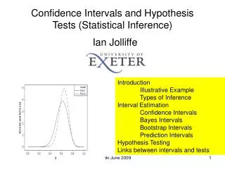
Assumptions for Z Confidence Intervals and Tests of Significance
Whenever we make a confidence interval or test of significance we must be certain that we meet theoretical assumptions before we may make the actual interval or test. Our tests and intervals cannot be applied to all circumstances. Fortunately, they do work in many circumstances, and we will be able to verify that this is so. The assumptions are the same for confidence intervals and tests of significance, so we have only one set to learn.
What if we don’t meet the assumptions? If we can tell from the problem statement or context that an assumption is not met, we must state so, and our results will be suspect. Due to the educational nature of this class, I will ask you to go ahead and work the problem, anyway, even if the assumptions are not met (but you must state that they are not met). In the real world, we would have to meet the assumption before proceeding, but because we are unable to redo an experiment, for example, we will use the information we have.
1st Assumption: The first assumption is that our sample is a simple random sample, usually abbreviated SRS. This information is usually provided in the problem. If so, we can simply state that SRS is given. Sometimes we will have no information about how the sample was made, and in that circumstance we can write that we are uncertain that we have an SRS.
If we can tell that our sample is not an SRS, we must state that. It may mean that our results are not valid. The simple random sample is so important because it avoids bias that may be the result of selection. Our sample should be representative of the population, otherwise we may draw conclusions about a group different from the one we wanted. Recall that randomization was an important principle of experimental design, and this is why! Randomization guarantees random samples.
2nd Assumption: The second assumption is that our sampling distribution is normally distributed. This assumption is met whenever our population is normally distributed. This information may be provided in the problem, and if so, we simply write that it is given that the population is normal. A principle that often helps us here, is the Central Limit Theorem. As sample size become large the sampling distribution approaches the normal distribution, even if the original population is not normal. When we have large samples, we invoke the CLT.
Otherwise, we must examine the data provided in an effort to see whether or not it is reasonable to expect the sampling distribution to be normal. We will spend more time on exactly what to do here later in the course.
3rd Assumption: Our third and final assumption is that is known. This must be provided to you in the problem, otherwise we cannot use the Z-interval or test. In Module 13, we will learn what to do when is unknown.
In summary: Whenever we perform statistical inference using a Z test or interval for sample means, we need: • SRS • Normal distribution of sampling distribution • (the population standard deviation)