Download
1 / 33
330 likes | 337 Views
Intro. to Neural Networks & Using a Radial-Basis Neural Network to Classify Mammograms. Pattern Recognition: 2 nd Presentation Mohammed Jirari Spring 2003. Neural Network History. Originally hailed as a breakthrough in AI

E N D
Intro. to Neural Networks& Using a Radial-Basis Neural Network to Classify Mammograms Pattern Recognition: 2nd Presentation Mohammed Jirari Spring 2003
Neural Network History • Originally hailed as a breakthrough in AI • Biologically inspired information processing systems (parallel architecture of animal brains vs processing/memory abstraction of human information processing) • Referred to as Connectionist Networks • Now, better understood • Hundreds of variants • Less a model of the actual brain than a useful tool • Numerous applications • handwriting, face, speech recognition • CMU van that drives itself
I1 W1 I1 W1 or W2 W2 O I2 O I2 W3 W3 I3 I3 Activation Function 1 Perceptrons • Initial proposal of connectionist networks • Rosenblatt, 50’s and 60’s • Essentially a linear discriminant composed of nodes, weights
2 .5 .3 =-1 1 Perceptron Example 2(0.5) + 1(0.3) + -1 = 0.3 , O=1 Learning Procedure: • Randomly assign weights (between 0-1) • Present inputs from training data • Get output O, nudge weights to gives results toward our desired output T • Repeat; stop when no errors, or enough epochs completed
Perception Training Weights include Threshold. T=Desired, O=Actual output. Example: T=0, O=1, W1=0.5, W2=0.3, I1=2, I2=1,Theta=-1
Perceptrons • Can add learning rate to speed up the learning process; just multiply in with delta computation • Essentially a linear discriminant • Perceptron theorem: If a linear discriminant exists that can separate the classes without error, the training procedure is guaranteed to find that line or plane.
Strengths of Neural Networks • Inherently Non-Linear • Rely on generalized input-output mappings • Provide confidence levels for solutions • Efficient handling of contextual data • Adaptable: • Great for changing environment • Potential problem with spikes in the environment
Strengths of Neural Networks (continued) • Can benefit from Neurobiological Research • Uniform analysis and design • Hardware implementable • Speed • Fault tolerance
Hebb’s Postulate of Learning “The effectiveness of a variable synapse between two neurons is increased by the repeated activation of the neuron by the other across the synapse” This postulate is often viewed as the basic principal behind neural networks
LMS Learning LMS = Least Mean Square learning Systems, more general than the previous perceptron learning rule. The concept is to minimize the total error, as measured over all training examples, P. O is the raw output, as calculated by E.g. if we have two patterns and T1=1, O1=0.8, T2=0, O2=0.5 then D=(0.5)[(1-0.8)2+(0-0.5)2]=.145 We want to minimize the LMS: C-learning rate E W(old) W(new) W
To compute how much to change weight for link k: Chain rule: We can remove the sum since we are taking the partial derivative wrt Oj LMS Gradient Descent • Using LMS, we want to minimize the error. We can do this by finding the direction on the error surface that most rapidly reduces the error rate; this is finding the slope of the error function by taking the derivative. The approach is called gradient descent (similar to hill climbing).
Activation Function • To apply the LMS learning rule, also known as the delta rule, we need a differentiable activation function. Old: New:
LMS vs. Limiting Threshold • With the new sigmoidal function that is differentiable, we can apply the delta rule toward learning. • Perceptron Method • Forced output to 0 or 1, while LMS uses the net output • Guaranteed to separate, if no error and is linearly separable • Gradient Descent Method: • May oscillate and not converge • May converge to wrong answer • Will converge to some minimum even if the classes are not linearly separable, unlike the earlier perceptron training method
Backpropagation Networks • Attributed to Rumelhart and McClelland, late 70’s • To bypass the linear classification problem, we can construct multilayer networks. Typically we have fully connected, feedforward networks. Input Layer Output Layer Hidden Layer I1 O1 H1 I2 H2 O2 I3 1 Wj,k Wi,j 1 1’s - bias
Backprop - Learning Learning Procedure: • Randomly assign weights (between 0-1) • Present inputs from training data, propagate to outputs • Compute outputs O, adjust weights according to the delta rule, backpropagating the errors. The weights will be nudged closer so that the network learns to give the desired output. • Repeat; stop when no errors, or enough epochs completed
Backprop - Modifying Weights We had computed: For the Output unit k, f(sum)=O(k). For the output units, this is: For the Hidden units (skipping some math), this is: I H O Wi,j Wj,k
Backprop • Very powerful - can learn any function, given enough hidden units! With enough hidden units, we can generate any function. • Have the same problems of Generalization vs. Memorization. With too many units, we will tend to memorize the input and not generalize well. Some schemes exist to “prune” the neural network. • Networks require extensive training, many parameters to fiddle with. Can be extremely slow to train. May also fall into local minima. • Inherently parallel algorithm, ideal for multiprocessor hardware. • Despite the cons, a very powerful algorithm that has seen widespread successful deployment.
Why This Project? • Breast Cancer is the most common cancer and is the second leading cause of cancer deaths • Mammographic screening reduces the mortality of breast cancer • But, mammography has low positive predictive value PPV (only 35% have malignancies) • Goal of Computer Aided Diagnosis CAD is to provide a second reading, hence reducing the false positive rate
Data Used in my Project • The dataset used is the Mammographic Image Analysis Society (MIAS) MINIMIAS database containing Medio-Lateral Oblique (MLO) views for each breast for 161 patients for a total of 322 images. Every image is: 1024 pixels X 1024 pixels X 256
Approach Followed: • Normalize all images between 0 and 1 • Normalize the features between 0 and 1 • Train the network • Test on an image (Simulate the network) • Denormalize the classification values
Features Used to Train • Character of background tissue: Fatty, Fatty-Glandular, and Dense-Glandular • Severity of abnormality: Benign or Malignant • Class of abnormality present: Calcification, Well-Defined/Circumscribed Masses, Spiculated Masses, Other/Ill-Defined Masses, Architectural Distortion, Asymmetry, and Normal
Radial Basis Network Used • Radial basis networks may require more neurons than standard feed-forward backpropagation FFBP networks • BUT, can be designed in a fraction of the time to train FFBP • Work best with many training vectors
radbas(n)=e^-(n^2) a=radbas(n)
Radial basis network consists of 2 layers: a hidden radial basis layer of S1 neurons and an output linear layer of S2 neurons:
Results and Future Work • The network was able to correctly classify 55% of the mammograms • I will use more pre-processing including sub-sampling, segmentation, and statistical features extracted from the images, as well as the coordinates of the center of abnormality and approximate radius of a circle enclosing the abnormality. • I will use different networks like fuzzy ARTMAP network, self-organizing network, cellular networks and compare their results in designing a good CAD.