Download
1 / 30
300 likes | 303 Views
Material Description of Ice in the Geophysical Context. Contents. 2.1 Constitutive relations for cold ice 2.2 The most simple 3D flow law for cold ice 2.3 Ice as a higher grade fluid 2.4 Constitutive relations of temperate ice in polythermal ice masses.

E N D
Material Description of Ice in the Geophysical Context Contents 2.1 Constitutive relations for cold ice 2.2 The most simple 3D flow law for cold ice 2.3 Ice as a higher grade fluid 2.4 Constitutive relations of temperate ice in polythermal ice masses
2.1 Constitutive relations for cold ice Definition: ● Ice, whose temperature is below the melting point, is called cold ice ● Ice of which the temperature is at the melting point is called temperate ice Polycrystal Representative Volume Element (RVE) Unit sphere for crystal orientations Schmidt circle Ice in glaciers and ice sheets is formed from falling snow flakes, subject to compression and sintering processes and with random orientations. At the surface, the orientation distribution of the crystals is randomly uniform. Consequences: ● Ice in glaciers and ice sheets is in first approximation an isotropic material ● At large depth, because of large deformations of the ice particles, the polycrystalline ice becomes anisotropic (see later)
a) Early experiments: Simple shear and uniaxial tension/compression at constant force (stress) or constant strain rate Simple shear Uniaxial tension/compression F ● For constant stress experiments - Applied force is monitored - Deformation (t), (t) is measured ● For constant strain rate experiments - Certain components of deformation are monitored - Forces are measured t
One differentiates: 1. Primary creep:Immediately after the stress/force is applied, strain sets in, growing in time, but with decreasing strain rate. This state is relatively short. 2. Secondary creep:In this regime, the strain grows approximately linearly, the strain rate is approximately constant. At small stresses, secondary creep lasts (infinitely) long (!!) 3. Tertiary creeparises at large stress; it is an accelerated creep process beyond secondary creep. It is always accompanied by stress- /strain induced crystallographic rearrangements (rotations, crystallizations). If the forces are moderate, tertiary creep goes over into stationary creep, if it is too strong, fracure or rupture occurs.
Plotting the displacement or strain or strain rate as a function of time the three regimes are easily identified. Important: Point of minimum creep rate Min. Creep rate At different stresses, the creep curves differ from one another as follows: Growing stress Postulate: The values of the stresses (deviators) in glaciers and ice sheets are so small that tertiary creep does not arise. Thus, one may replace the true creep curves by those of minimal creep. This statement is no longer accepted.
Measured creep curves Mellor & Testa (1971) Creep curves at small stresses for small-grained ice with initially statistically uniform orientation distribution Glen 1953 Glen 1953 Creep curves for isotropic polycrystalline ice for different stresses Creep curves for isotropic polycrystalline ice at various temperatures at a pressure of 6X10⁵Pa
To make tertiary creep visible one must scale such that primary creep is hardly visible any longer Steinemann (1958) Creep curves for isotropic polycrystalline ice at -4.8°C at high stresses (in bar) Based on such experiments various constitutive relations have been proposed. 1. Reproduction of all creep regimes. Then generalization to 3D. → Morland & Spring (1980/81). This is unsatisfactory. 2. Reproduction of primary and secondary creep. Good for small stresses and short time processes. McTigue, Jones, Passman (1981), Man & Sun (1982) 3. Reproduction to stationary secondary creep → Glen´s flow law and its generalization
Construction of a flow law For different temperatures, one determines the curves , a popular fit to the curves is (*) temperature dependent rate factor creep response function Remarks: ● If f(||)= ||n, then (*) is called a power law. In Glaciology the power law is called Glen’s flow law, but in materials science and rheology it is referred to as Norton, Graham, Gang, Oswald & de Waele, Reiner-Rivlin law, etc. ● I propose to call it in glaciology the Glen-Steinemann law ● In analogy to this I shall call (*) with a general creep response function the generalized Glen flow law
The power law is not optimal Stationary creep rates under secondary creep for polycrystalline ice in doubly log representation are not straight linear curves (Steinemann, 1958) Steinemann´s parameterization (**) Arrhenius law Boltzmann constant Abs. temperature Secondary creep Activation energy Tertiary creep
Remarks: ● Steinemann´s experiments show that n = n(). So, (**) is not a power law ● Apparently Glen´s experiments were not accurate enough, since Glen´s n is not stress dependent. Glen´s value of n over all his experiments is n = 3.5. However, glaciologists use worldwide ● The Arrhenius law matches experiments only for T< 263 K. For T > 263 K it is not the best fit. However, this regime is glaciologically important. n = 3 (secondary creep) Stationary creep rate for tertiary creep of poly crystalline ice as a function of stress (Steinemann)
Other rate factor representations ● Patching two Arrhenius relations together This parameterization has a kink at T = 263K ● Spline interpolations of pointwise-determined rate factors for different temperatures for 210K < T < 273.15K ● It is important to write the flow law in terms of a „homologous“ temperature Morland & Smith (1985) have parameterized the data of Meller & Testa as follows:
Remark: Generally, in data from different ice sheets, absolute values of A differ from one another. This is indication that some micro-dependencies are ignored. Other creep functions ● Glen´s flow law has an infinite slope, (for n > 1) at zero strain rate (or zero stress (deviator)). For very small strain rates Glen´s flow law has therefore infinitely large viscosity at zero strain rate. This causes mathematical difficulties. ● For n = 1 Glen´s flow law reduces to that of a Newtonian fluid (Navier- Stokes fluid) ● Most alternative laws that are proposed by experimental glaciologists, however, also have infinite viscosity at zero strain rate.
Glen-Steinmann law is singular (1953,1958) Lliboutry 1969 (regular for A0 0) Colebeck & Evans (1973), Thompson (1979), Hutter (1980) (regular for k 0) Prandtl-Eyring, regular → Barnes et al. (1973), singular Carofalo
The best agreement is obtained with the Garofalo law, as introduced by Barnes et al. However, this law has infinite viscosity at zero strain rate. Hutter (1983) proposed to complement this law with a linear term. Then it reads (precent/s) regularizes the law:
Experimental fit by the Garofalo law (1971) with changes).
Remarks: ● Because of the large scatter of the experimental results between specimens from different locations and at different temperatures, it is relatively unimportant which parameterization is used. ● Laws with are called infinite viscosity laws. ● Glaciologists tried to correlate Glen´s flow law by field measurements (Hooke, 1981). This is problematic, since external loads cannot be controlled, so that ad-hoc assumptions are needed. An improvement of the creep response function from the power law is not possible; the exponent is hardly identifiable. ● Laboratory experiments are always performed at much larger stresses than those occurring in Nature, since experiments must be completed in a human´s life time. So, can such experiments be representative for ice in Nature?
2.2 The most simple 3D flow law for cold ice Postulate: Cold ice in glaciers and ice sheets is a density preserving, viscous heat conducting fluid This implies for the internal energy, the heat flux vector and the stress tensor the following constitutive relations On phase change surfaces (reversible surfaces, [[p]] = 0, [[T]] = 0, [[v]] = 0) L: latent heat
Remarks: ● The law (*) is, relative to a general isotropic representation, already simplified. The dependence of the heat conductivity on temperature should not be ignored. ● In Glaciology enthalpy formulations are preferred to free energy formulations → ● Parameters for the general isotropic stress representation cannot be identified only with {uniaxial tension/compression} experiments. That such experiments suffice, additional simplifying assumptions must be made, which may be questionable.
Nye´s 3D generalization of Glen´s flow law Assumption 1: In the stress relation the dependence on the temperature gradient can be dropped, since such a dependence has never been measured. So, () Moreover, since for density preserving fluids trD = ID = 0, equation must satisfy the deviator relation
Assumption 2: D and TD are affine to each other. → 3 = 0. (Stress and stretching are collinear) Assumption 3: D does not depend on the third stress deviator invariant. So, (Note ITD= 0) Assumption 4: The function B = B(IITD,T)can be factorized as follows It follows, the 3D generalization of the generalized Glen´s flow law is given by The coefficients A(T) and f(IITD) must be identified by experiments. Glaciologists use ● Uniaxial tension/compression tests ● Simple shear tests, Couette viscometric experiments ● Bore hole deformation measurements
1. Simple shear Simple shear allows direct determination of the functions A(T) and f(IITD) .
2. Uniaxial compression/tensile stresses Thus, the flow law for uniaxial compression is Experimentally A(T) and f(IITD) are determined. Then
Remarks: ● Assuming a Reiner-Rivlin fluid relation, Glen demonstrated in 1958 on the basis of the data by Steinemann that in 3D Nye´s form of the stress relation D = A(T)f(IITD)TD, is not well matched by his experiments concerning shear and compression. ● If the generalized Glen flow law, D = A(T)f(IITD)TDis inverted, then no product representation between temperature and stretching dependent functions is obtained unless f(.) is a power function. In fact, It is obvious from the above relation that the power law yields in the inverted version again a product seperation.
2.3 Ice as a higher grade fluid ● Nye´s 3D form of Glen´s flow law can only describe stationary creep. The complete behaviour, however, should include primary, secondary and tertiary creep. - Nye´s flow law does not allow Normal Stress Effect. Some experiments seem to suggest them to be present in ice flow. According to these, normal stress effects are accompanied with dilatancy. With snow, which is a granular porous material, this is better understood. - Primary and secondary creep, but not tertiary creep, can be modeled as follows (1) Ice is a simple fluid of second order with constant coefficients. This law has been proposed by McTigue, Passman & Jones (J. Glac. 31, 1985, 108). It can not be reduced to Glen´s flow law.
(2) Man & Sun [J. Glac. 33, 1987, 268-273] proposed instead Man & Sun call (1) „Modified second order flow law with power law viscosity“ and (2) a „Power law fluid of grade 2“. For m = (1-n)/n and 1 = 2 = 0, Glen´s law emerges Both author teams identify the free coefficients with laboratory experiments. However, no tertiary creep can be modeled. For engineering processes and fluid behaviour this may be acceptable. For ice flow in large ice masses, it is the wrong approach.
2.4 Constitutive relations of temperate ice in polythermal ice masses Polythermal ice masses consist of disjoint regions with cold and temperate ice, respectively. Definition:Temperate ice is a mixture of ice and water inclusions, where both ice and water are at the melting point. cold ice The water inclusions are partly connected along the grain boundaries. Thus, the water can diffusively move, if, however, only very slowly. temperate ice Definition: Let wand be the mass densities for the water and the ice-water mixture. The variable is called the moisture content of temperate ice. The moisture content in the temperate ice of polythermal ice masses is 3 – 5 %, no more!
Postulate: The temperate ice in polythermal ice masses is a binary mixture of ice + water with isolated and connected inclusions. Remarks: ● The masses of the constituents ice and water are significant, since water diffuses through the „ice matrix“. ● Momentum is balanced for the mixture as a whole. So v is the barycentric velocity and the mixture density. ● The mixture energy equation does not determine the temperature, which is at the melting point, but it rather serves as an equation that determines the production of water by the melting and freezing processes. Assumption: The mixture can be treated as incompressible.
Field equations (moisture content) Postulate: The binary mixture of temperate ice in polythermal ice masses can be treated as a viscous heat conducting Newtonian-Fourier-Fick fluid with Glen-type constitutive relation for the stress.
Thermodynamics then show Remarks: ● The rate factor is now a function of the moisture content and not the temperature (which is given by the Clausius-Clapeyron equation) ● It is assumed that the free energy or enthalpy do not depend on the moisture content, Then the Gibbs relation reduces to and the Clausius-Clapeyron equation becomes where T is always the freezing/melting temperature. So
Expression for the internal energy of temperate ice Entropy Internal energy Thus, the energy equation becomes and mass balance for the water reduces to → So: