Download
1 / 26
260 likes | 271 Views
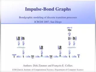
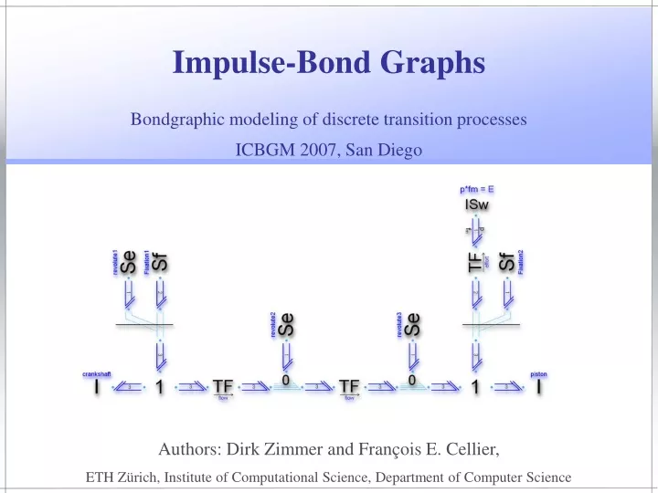
Authors: Dirk Zimmer and François E. Cellier, ETH Zürich, Institute of Computational Science, Department of Computer Science. Impulse-Bond Graphs. Bondgraphic modeling of discrete transition processes ICBGM 2007, San Diego. Overview. Motivation Definition of impulse bonds

E N D
Authors: Dirk Zimmer and François E. Cellier, ETH Zürich, Institute of Computational Science, Department of Computer Science Impulse-Bond Graphs Bondgraphic modeling of discrete transition processes ICBGM 2007, San Diego
Overview • Motivation • Definition of impulse bonds • Mechanical impulse-bond graphs • Derivation of an IBG from a regular BG • Limitations • Conclusions
Motivation I • Impulse Bond Graphs (IBGs) have been primarily developed to describe discrete transition processes in mechanical systems. • Such transitions usually represent elastic or semi-elastic collisions. In these cases, the transition model is an intermediate model that interrupts the continuous process. • Discrete transitions might also represent non-elastic collisions (for instance a transition from friction to stiction). Such transitions are typically reducing the degrees of freedom in the overall system. Hence they represent a transition between two different continuous modes.
Motivation II • Since normal bonds describe a continuous process, they are obviously unable to describe a discrete transition. • In general, we observe that a discrete change of a bondgraphic variable (effort, flow) is accompanied by an impulse quantity of its dual counterpart. • Based on this observation we developed a new type of bonds that enables us to represent a transition model in a bondgraphic fashion. We call these bonds: Impulse bonds. • Although impulse bond graphs (IBGs) are primarily intended for mechanical system, they can be embedded into the general bondgraphic framework.
Impulse Bonds. • An impulse bond is a pseudo-bond, where the product of the adjugated variables represents an amount of work. It is represented by a two-headed harpoon: • The regular impulse bond describes an impulse of effort p that leads to a sudden change of flow f from fpre to fpost, where fm = (fpre+fpost)/2. • Hence an impulse bond represents a sudden transmission of energy between its vertex elements and not a continuous power flow.
Impulse Bonds. • It is a prerequisite for any kind of impulse modeling that the integral curve of e is irrelevant. Hence we can suppose e to be of rectangular shape. • We suppose, that the impulse relevant storage and transformation elements are all linear. Hence the flow f is linearly changing. • The work W is the integrated power curve and can now be transformed into the product W = p · fm , where • p = ∫e dt • fm= (fpre+ fpost)/2
First Example • Let us model the elastic collision between two rigid bodies in a mechanical system. • The model structure before and after the collision is not affected. The continuous part can therefore sufficiently be described by a single bond-graph. • The collision causes an impulse of force that leads to a discrete change of velocity. This transition is modeled by the corresponding impulse-bond graph.
1st Example: Continuous Model • The gravity affects only the vertical domain. • The collision affects only the horizontal domain. • The corresponding transformers are modulated by the pendulum angle. • The position sensor Dq triggers the collision.
1st Example: Transition Model • This impulse bond graph represents a linear system of equations. • The impulse is triggered by the impulse switch element ISw: fm = 0 : at the time of collision. p = 0 : otherwise. • This specific switch is neutral with respect to energy since the product p·fm is always zero. • In general, impulse switches can dissipate or sometimes even generate energy.
1st Example: Transition Model • Obviously, the impulse bond graph inherited its structure from its continuous parent model. • A small number of fixed conversion rules enables the modeler to derive the IBG from an existing regular BG in a convenient way. • This allows a modeler to automatically transfer the knowledge contained in the regular BG to the corresponding IBG.
Derivation Rules I • Effort sources, capacitive and resistive elements do neither cause nor transmit any effort impulse and can therefore be neglected if they are connected to a 1-junction. If they are connected to a 0-junction, they have to be replaced by a source of zero effort. • All sensor elements can be removed.
Derivation Rules II • All junctions remain. • Sources of flow determine the flow variable and consequently also the average flow variable fm.Therefore these elements remain unchanged. • Linear transformers or gyrators also project the impulse variable and the average by the same linear factor. Thus, also these elements remain unchanged.
Derivation Rules III • All modulating signals must be replaced by a constant signal for the time of the impulse. Hence modulated transformers must become linear transformers. • Inductances or inductive fields are still denoted by the same symbol, but they represent now different equations. • Finally, one needs to include the ISw Element. • The resulting IBG can than be simplified.
2nd Example • Let us create a simple, academic model of a piston engine. • This is a planar mechanical model that includes a kinematic loop: There are 4 joints that each define one degree of freedom, but the final model owns only one degree of freedom. • The ignition is triggered when the piston’s position reaches a certain threshold. • The ignition is regarded as a discrete event that causes a force impulse so that each ignition will add a constant amount of energy into the system.
2nd Example • The model below represents the continuous part, and has been created with components that contain wrapped planar mechanical multi-bond graphs: • The components feature icons that make the model intuitively understandable.
2nd Example • Unwrapping the model leads to a multi-bond graph. The unwrapping is not necessary for simulation, it is only done here to reveal the underlying bondgraphic model. • The multi-bond graph uses planar mechanical multi-bonds, where the first two components belong to the translational domain, and the third component describes the rotational domain. All variables are resolved with respect to the inertial system. • Whereas the bond graph cares about the dynamics, the signals care about the positional state of the system.
2nd Example r = fixed r { = fixed 0 { a a b b , 0 0 a a b b a , } 0 spring } c = 0 a b revolute a prismatic n = { 1 , b 0 } b
2nd Example: Results • The ISw elements contains a non-linear equation: • p ·| fm| = Eexplosion : at the time of ignition. • p = 0 : otherwise. Hence, this IBG describes a non-linear system of equation. • Dymola reduces the systemto a size of 10. The corres-ponding simulation result is shown on the right. The plot displays the angular velocity
Linearity • An IBG must consist of linear elements to be valid. The only exception is the ISw element. • Otherwise the product of the adjugated variables would not represent the correct amount of work anymore. • Fortunately, all mechanical IBGs are linear, because all potential non-linear elements of the continuous domain vanish. • Non-linear capacitances and resistances disappear • Non-linear modulation by position becomes constant. • The inductance are always linear (Newton’s law)
Non-linearities • Impulse modeling on non-linear storage elements is principally possible, but the usability of IBGs is drastically impaired. • The product of the adjugated variables becomes meaningless • Junctions cannot be considered to be energy neutral anymore. • Transformers elements must be linear to enable impulse modeling in general. • Non-linear storage elements must be integrable into the form: fpost = h(p,fpre), where h is a non-linear function.
Other domains • One can define impulse bonds also for other domains. This generates the need for dual type of impulse bonds. • Hence, one distinguishes between the effort impulse bond and the flow impulse bond: • The flow impulse bond can be used for instance in electric circuits to represent an impulse of current, i. e. a transmission of charge.
Conclusions I • Impulse-bond graphs have been applied for the development of the MultiBondLib. The MultiBondLib is a free Modelica Library for general multi-bond graphs. • The library additionally contains also mechanical components based upon wrapped MBGs. Especially an extensive set of hybrid mechanical components is provided. • The corresponding impulse-equations of these hybrid components have been derived by the methodology of impulse-bond graphs. • Originally it was intended to wrap the graphical models of the BG and the IBG together, but this caused practical difficulties, since the two graphical models obstructed each other.
Conclusions II • IBGs represent a convenient way to describe discrete transition processes in a bondgraphic fashion. They are especially suited for mechanics. • We think that IBG are valuable for the understanding and teaching of discrete transition processes in physical systems. • The derivation rules enable a convenient transfer of knowledge. • Currently we do not provide an implementation for IBGs that is able to conveniently interact with its continuous parent model. Hence impulse-bond graphs remain purely a modeling tool so far. • The restriction to linear elements impairs the generality of IBGs in non-mechanical domains.