Download
1 / 35
350 likes | 359 Views
This article discusses linear methods for regression, particularly their performance when n is small, p is large, and/or the noise variance is large. It covers the model, estimation of parameters, prediction, hat matrix, degrees of freedom, inference, and testing of null hypotheses. Additionally, it explores the concept of confidence regions for parameters. The prostate cancer dataset is used as an example.

E N D
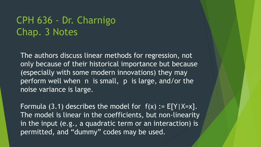
CPH 636 - Dr. CharnigoChap. 3 Notes The authors discuss linear methods for regression, not only because of their historical importance but because (especially with some modern innovations) they may perform well when n is small, p is large, and/or the noise variance is large. Formula (3.1) describes the model for f(x) := E[Y|X=x]. The model is linear in the coefficients, but non-linearity in the input (e.g., a quadratic term or an interaction) is permitted, and “dummy” codes may be used.
CPH 636 - Dr. CharnigoChap. 3 Notes Because f(x) is linear in the parameters (β0, β1, …, βp), estimating the parameters by ordinary least squares – i.e., minimization of (3.2) – leads to the closed-form solution in (3.6). While I won’t show you a proof of the general case, which entails vector calculus and linear algebra, I will show you how the solution is obtained with p=1 and neglecting the intercept.
CPH 636 - Dr. CharnigoChap. 3 Notes Note that, once the parameters are estimated, we may predict Y for any x. In particular, (3.7) shows that predicting Y for x which occurred in the training data is accomplished by a matrix-vector multiplication, Ypredicted = HYtraining, where H := X(XTX)-1XT. To make predictions for a new data set (rather than for the training data set), replace the first X in H by its analogue from the new data set.
CPH 636 - Dr. CharnigoChap. 3 Notes We refer to H as the hat matrix. The hat matrix is what mathematicians call a projection matrix. Consequently, H2= H. Figure 3.2 provides an illustration with p=2, but I will provide an illustration with p=1 which may be easier to understand. Assuming there are no redundancies in the columns of X, the trace of H is p+1. This trace is called the degrees of freedom (df) for the model, a concept which generalizes to nonparametric methods which are linear in the outcomes.
CPH 636 - Dr. CharnigoChap. 3 Notes If we regard the predictors as fixed rather than random (or, if we condition upon their observed values), then under the usual assumptions for linear regression (what are they ?), we have result (3.10). Combined with result (3.11), which says that the residual sum of squares divided by the error variance follows the chi-square distribution on n-p-1 degrees of freedom, result (3.10) forms the basis for inference on β0, β1, …, βp. (Even if we are more interested in prediction, this is still worth your understanding.)
CPH 636 - Dr. CharnigoChap. 3 Notes The authors make the point that the T distribution which is proper to such inferences is often replaced by the Z distribution when n (or, rather, n-p-1) is large. I think that the authors have oversimplified a bit here, though, because the adequacy of the Z approximation to the T distribution depends on the desired level of confidence or significance. In any case, with modern computing powerful enough to implement methods in this book, why use such an approximation at all ?
CPH 636 - Dr. CharnigoChap. 3 Notes Result (3.13) tells you how to test a null hypothesis that some but not all predictors in your model are unnecessary. This is important because testing H0: β1 = β2 = 0 is not the same as testing H0: β1 = 0 and H0: β2 = 0. Possibly X1 could be deleted if X2 were kept in the model, or vice versa, while deleting both might be undesirable. For example, consider X1 = SBP and X2 = DBP.
CPH 636 - Dr. CharnigoChap. 3 Notes One could (and sometimes does, especially in backward elimination) test whether to remove X2 and then, once X2 is gone, test whether to remove X1 as well. But that entails sequential hypothesis testing, which is not simple in terms of its implications for actual versus nominal significance level. Moreover, there are some situations in which X1 and X2 should either both or neither be in the model, such as when they are dummy variables.
CPH 636 - Dr. CharnigoChap. 3 Notes Result (3.15) describes how to make a confidence region for β0, β1, …, βp. I will illustrate what this looks like for β0 and β1 when p = 1. Importantly, such a region is not a rectangle. Though not shown explicitly in (3.15), one may also make a confidence region for any subset of the parameters. I will illustrate what this looks like for β1 and β2 when p > 2 supposing that, for example, X1 = SBP and X2 = DBP.
CPH 636 - Dr. CharnigoChap. 3 Notes The authors discuss the prostate cancer data set at some length. Notice that they began (Figure 1.1) by exploring the data. The authors identify the “strongest effect” as belonging to the input with the largest Z score. This seems to conflate the magnitude of effect of the input on the mean output level with the degree of conviction that the magnitude is nonzero.
CPH 636 - Dr. CharnigoChap. 3 Notes Let’s also make sure we understand what the authors mean by “base error rate” and its reduction by 50%. Returning to the idea of inference, the Gauss-Markov Theorem indicates that, for a correctly specified model: (i) parameters are estimated unbiasedly; and, (ii) parameters are estimated with minimal variance subject to (i).
CPH 636 - Dr. CharnigoChap. 3 Notes Although the Gauss-Markov Theorem sounds reassuring, there are some cases when we can achieve a huge reduction in variance by tolerating a modest amount of bias. This may substantially reduce both mean square error of estimation and mean square error of prediction. Moreover, there’s a big catch to the Gauss-Markov Theorem: for a correctly specified model. There are many ways that a model specification can be incorrect.
CPH 636 - Dr. CharnigoChap. 3 Notes The authors proceed to describe how a multiple linear regression model can actually be viewed as the result of fitting several simple linear regression models. They begin by noting that when the inputs are orthogonal (roughly akin to the idea of statistical independence), unadjusted and adjusted parameter estimates are identical.
CPH 636 - Dr. CharnigoChap. 3 Notes Usually inputs are not orthogonal. But imagine that, with standardized inputs and response (hence, no need for an intercept), we do the following: • Multiple linear regression of Xk on all other features. • Simple linear regression of Y on the residuals from step 1. These residuals are orthogonal to the other features…
CPH 636 - Dr. CharnigoChap. 3 Notes …and so the parameter estimate from step 2 will be the same as we would have obtained for Xk in a multiple linear regression of Y on X1, X2, …, Xp. This gives us an alternate interpretation of an adjusted regression coefficient: we are quantifying the effect of Xk on that portion of Y which is orthogonal to (or, if you prefer, unexplained by) the other inputs.
CPH 636 - Dr. CharnigoChap. 3 Notes Formula (3.29) then shows why it’s difficult to estimate the coefficient for Xk if Xk is strongly linearly related to the other features, a phenomenon known as (multi)collinearity. The denominator of (3.29) is also related to the variance inflation factor, a diagnostic for collinearity.
CPH 636 - Dr. CharnigoChap. 3 Notes You may have also heard of the distinction between ANOVA and MANOVA. You may wonder, then, whether there is an analogue to MANOVA for situations when you have multiple continuous outcomes which are being regressed on multiple continuous predictors.
CPH 636 - Dr. CharnigoChap. 3 Notes There is, but parameter estimates relating a particular outcome to the predictors do not depend on whether they are acquired for the one outcome by itself or for all outcomes simultaneously. This is true even if the multiple outcomes are correlated with each other. This is in stark contrast to the dependence of parameter estimates relating a particular outcome to a particular predictor on whether other predictors are considered simultaneously.
CPH 636 - Dr. CharnigoChap. 3 Notes The authors suggest that ordinary least squares may have more variability than bias. (Here they assume that the model is specified correctly. If the model is a drastic simplification of reality, then ordinary least squares may have more bias than variability, especially versus competing approaches to statistical learning.) The authors therefore discuss subset selection, which may reduce variability (though increase bias) and enhance interpretation.
CPH 636 - Dr. CharnigoChap. 3 Notes Best subset selection, which is computationally feasible for up to a few dozen candidate predictors, entails finding the best one-predictor model, the best two-predictor model, and so forth. This is illustrated in Figure 3.5. Then, using either a validation data set or cross-validation (the authors do the latter in Figure 3.7), choose from among the best one-predictor model, best two-predictor model, and so forth.
CPH 636 - Dr. CharnigoChap. 3 Notes Note that the authors do not define “best” strictly by mean square error of prediction but also by considerations of parsimony. Forward selection is an alternative to best subsets selection when p is large. The authors refer to it as a “greedy algorithm” because, at each step, that predictor is chosen which explains the greatest part of the remaining variability in the outcome.
CPH 636 - Dr. CharnigoChap. 3 Notes While that seems desirable, the end result may actually be sub-optimal if predictors are strongly correlated. Backward elimination is another option. A disadvantage is that it may not be viable when p is large relative to n. A compelling advantage is that backward elimination can be easily implemented “manually” if not otherwise programmed into the statistical software. This may be useful in, for example, PROC MIXED of SAS.
CPH 636 - Dr. CharnigoChap. 3 Notes In addition to explicitly choosing from among available predictors, we may also employ “shrinkage” methods for estimating parameters in a linear regression model. These are so called because the resulting estimates are often smaller in magnitude than those acquired via ordinary least squares. For the rest of these slides, we assume that Y and X1, …, Xp are standardized (with respect to training data).
CPH 636 - Dr. CharnigoChap. 3 Notes Ridge regression is defined by formula (3.44) in the textbook and can be viewed as the solution to the penalized least squares problem expressed in (3.41). Though perhaps not obvious, the constrained least squares problem in (3.42) is equivalent to (3.41), for an appropriate choice of t depending on λ. Moreover, (3.44) may be a good way to address collinearity. In particular, a correlation of ρ between X1 and X2 is, roughly speaking, reduced to ρ / (1 + λ).
CPH 636 - Dr. CharnigoChap. 3 Notes Figure 3.8 displays a “ridge trace”, which shows how the estimated parameters in ridge regression depend on λ. One may choose λ by cross validation, as the authors have done. Ridge regression can also be viewed as finding a Bayesian posterior mode (while ordinary least squares corresponds to frequentist maximum likelihood), when the prior distribution on each estimated parameter is normal with mean 0 and variance σ2 / λ.
CPH 636 - Dr. CharnigoChap. 3 Notes Ridge regression moves toward the “bias” side of the bias/variance tradeoff, versus ordinary least squares. One weakness of ridge regression is that, almost invariably, you retain all of the inputs. Even if the collinearity issue is resolved, why is this a weakness ? An alternative is the lasso, for which the corresponding optimization problems are (3.51) and (3.52).
CPH 636 - Dr. CharnigoChap. 3 Notes There is no analytic solution for the parameter estimates with the lasso; one must use numerical optimization methods. However, a positive feature of the lasso is that some parameter estimates are “shrunk” to zero. In other words, some variables are effectively removed. Figure 3.10 displays estimated parameters in relation to a shrinkage factor s which is proportional to t.
CPH 636 - Dr. CharnigoChap. 3 Notes Figure 3.11 explains why the lasso can effectively remove some predictors from the model. Each red ellipse represents a contour on which the residual sum of squares equals a fixed value. However, we are only allowed to accept parameter estimates within the blue regions. So, the final parameter estimates will occur where an ellipse is tangent to a region. For a circular region, this will almost never happen along a coordinate axis.
CPH 636 - Dr. CharnigoChap. 3 Notes The lasso also has a Bayesian interpretation, corresponding to a prior distribution on parameter estimates which has much heavier tails than a normal distribution. Thus, the lasso is less capable of reducing very large ordinary least squares estimates such as may occur with collinearity. Table 3.4 characterizes how subset selection, lasso, and ridge regression shrink ordinary least squares parameter estimates for uncorrelated predictors.
CPH 636 - Dr. CharnigoChap. 3 Notes While having uncorrelated predictors is a fanciful notion for an observational study (versus a designed experiment), Table 3.4 helps explain why ridge regression does not produce zeroes and why the lasso is more of a “continuous” operation than subset selection. The authors also mention the elastic net and least angle regression as shrinkage methods.
CPH 636 - Dr. CharnigoChap. 3 Notes The former is a sort of compromise between ridge regression and the lasso, as suggested by Figure 18.5 later in the textbook. The idea is to both reduce very large ordinary least squares estimates and eliminate extraneous predictors from the model. The latter is similar to the lasso, as shown in Figure 3.15, and provides insight into how to compute parameter estimates for the lasso more efficiently.
CPH 636 - Dr. CharnigoChap. 3 Notes Besides subset selection and shrinkage methods, one may fit linear regression models via approaches based on derived input directions. Principal components regression replaces X1, X2, …, Xp by a set of uncorrelated variables W1, W2, …, Wp such that Var(W1) >Var(W2) > … >Var(Wp). Each W is a linear combination of the X’s, such that the squared coefficients of the X’s sum to 1.
CPH 636 - Dr. CharnigoChap. 3 Notes One then uses some or all of W1, W2, …, Wp as predictors in lieu of X1, X2, …, Xp. This eliminates any problem that may exist with collinearity. The downside of principal components regression is that a W may be difficult to interpret, unless it should happen that the W is approximately proportional to an average of some of the X’s or a “contrast” (the difference between the average of one subset of the X’s and the average of another subset).
CPH 636 - Dr. CharnigoChap. 3 Notes Partial least squares – which has been investigated by our own Dr. Rayens, among others - is similar to principal components regression, except that W1, W2, …, Wp are chosen in a way that Corr2(Y,W1)Var(W1) > Corr2(Y,W2)Var(W2) > … > Corr2(Y,Wp)Var(Wp). If one intends to use only some of W1, W2, …, Wp as predictors, partial least squares may explain more variation in Y than principal components regression.
CPH 636 - Dr. CharnigoChap. 3 Notes Figure 3.18 compares ordinary least squares, best subset selection, ridge regression, lasso, principal components regression, and partial least squares. To aid in the interpretation, note that X2 could be expressed as + or - (1/2) X1 + (sqrt(3)/2) Z, where Z is standard normal and independent of X1. Also, W1 = (X1 + or - X2) / sqrt(2) and W2 = (X1 – or + X2) / sqrt(2) for principal components regression.