Download
1 / 39
410 likes | 667 Views
A way of understanding diffusion: Random Walk. Spread of molecules from one spot is proportional to square root of time for random walk. Therefore, to go 2X as far takes 4X as long. A way of understanding diffusion: Fick’s Law. J is flux. D is diffusion constant. is concentration.

E N D
A way of understanding diffusion: Random Walk Spread of molecules from one spot is proportional to square root of time for random walk. Therefore, to go 2X as far takes 4X as long.
A way of understanding diffusion: Fick’s Law • J is flux • D is diffusion constant • is concentration
Diffusion Constant: What controls it? • Random thermal motions: D = kTv/f • f depends on size of particle and viscosity of solution. Spheres: scale as m1/3 (radius scaling)
Cartoon of FRAP Bleach creates “hole” of fluorophores, Diffusion is measured by “hole filling in” Bleach high power Monitor low power
Analysis of membrane compartments Cells expressing VSVG–GFP were incubated at 40 °C to retain VSVG–GFP in the endoplasmic reticulum (ER) under control conditions (top panel) or in the presence of tunicamycin (bottom panel). Fluorescence recovery after photobleaching (FRAP) revealed that VSVG–GFP was highly mobile in ER membranes at 40 °C but was immobilized in the presence of tunicamycin(Nehls et al, 2000 Nature Cell Biology)
Experimental Setup • Laser beam focused or through small field diaphragm • Rapid shutter to switch from high powered beam for bleach to attenuated beam for recovery same power won’t work-Keep bleaching) • Detector: PMT, camera ? • Original apparatus used stationary laser spot (still sometimes used) • Later improvement included scanning mirror to scan spot over sample. • Now can be done with laser scanning confocal instruments. (for some cases-e.g. membranes)
Y X = mobile fraction Idealized photobleaching data D =w2/4D
More Diffusion types Fully recovers Important for Large macromolecules: Collisions, obstacles, binding
Binding to immobilized matrix will reduce fraction of molecules diffusing B Both A and B will have similar D in Membrane although Very different sizes A intra extracellular
Diffusion of membrane components can be seen as a two dimensional diffusion problem • Membrane is modeled as infinite plane • Viscosity of the lipid bilayer is ~ 2 orders of magnitude higher than water • As shown by Saffman and Delbruck, the translational diffusion coefficient for membrane components depends only on the size of the membrane spanning domain
Spot Photobleaching • Bleach and monitor single diffraction limited spot • Assumes infinite reservoir of fluorescent molecules (hole can fill back in) • Use D = w2/4D to obtain D • Determine w = nominal width of Gaussian spot by other optical method 1/e2 point • Fit fluorescence recovery curve to obtain D Axelrod et al., 1976
PSF and Beam Waist Imaging sub-resolution 100 nm fluorescent beads Use 1/e2 points to get ωbeam waist (87%) D =w2/4D
Note that beam is still Gaussian Line scan of single points F x Different bleaching geometries yield different types of information • Line photobleaching generates a one-dimensional diffusion problem Allows collection of more fluorescence, averaging
where ais a constant reflecting extent of bleaching. Koppel, 1979 Biophys. J. 281 Scanning over bleach spot improves ability to characterize recovery curves • Allows accurate characterization of the bleach geometry and size for each individual experiment • Simplifies fits of recovery curves to: • Allows compensation for photobleaching during monitoring and sample drift.
Different bleaching geometries yield different types of information No recovery Recovery Pre-bleach image Photobleach Post-bleach image
FRAP of GFP in Mitochondria Fast limit: cytoplasm Slow limit: membrane bound Suggests barriers (cristae) need to be large Occlude 90% space Verkman, TIBS, 2002
Size dependence of dextrans (polysaccharides) diffusion in solution Not simple spheres: Random coils No simple m1/3 scaling Verkman, J. Cell Biology 1999
Diffusion of FITC Dextrans, Ficolls in MDCK Cell Cytoplasm Heavy dextrans very slow Mobile fraction low: binding More polarizable Verkman, J. Cell Biology 1999
FRAP in Cytoplasm • Problem is much more complicated because of three dimensional freely diffusing geometry.
Problems with FRAP of cytoplasmic components (2 orders of magnitude fasterthan membranes) 1. Diffusion is fast compared to bleaching and monitoring rate D=ms : cannot truly scan 2 If use small bleach regions, redistribution may occur during bleaching. In fact, often cannot observe bleach of small region at all. 3. By enlarging the size of the bleach region, can overcome this problem: but lose localization
Photobleaching of cytoplasmic components • One solution is to measure cytoplasmic diffusion by comparing to characteristic times of known samples in solutions of known viscosity. • e.g. Luby-Phelps et al., 1994. • SekSek et al. 1997. • D = kT/f • Not reliable, cytoplasm complicated collection of fluid, cytoskeletal components, endosome, etc: simple viscosity not sufficient D =w2/4D
Low NA lens Photobleaching of cytoplasmic components Another solution is to use geometry such depth of field is comparable to thickness of cell High NA lens Recovery is convolved With depth of field Geometry approximates cylinder bleached through Z Diffusion becomes 2D problem: easier
Multiphoton bleaching Need 3D treatment
Determination of Point Spread Function of Microscope 175 nm Bead Sub-resolution Volume is Ellipsoid Axial ~NA2
Typical 2-photon Photobleaching setup (Point Bleach) Controls power 1-p would need pinhole Bleach high power Monitor low power ~20% for 2-p
Fluorescence Loss in Photobleaching “FLIP”continuous bleaching measure of mobility Figure 3 | Fluorescence loss in photobleaching. Protein fluorescence in a small area of the cell (box) is bleached repetitively. Loss of fluorescence in areas outside the box indicates that the fluorescent protein diffuses between the bleached and unbleached areas. Repetitive photobleaching of an endoplasmic reticulum (ER) GFP-tagged membrane protein reveals the continuity of the ER in a COS-7 cell. Image times are indicated in the lower right corners. The postbleach image was obtained immediately after the first photobleach. The cell was repeatedly photobleached in the same box every 40 s. After 18 min, the entire ER fluorescence was depleted, indicating that all of the GFP-tagged protein was highly mobile and that the entire ER was continuous with the region in the bleach box. (Nehls et al, 2000 Nature Cell Biology)
Photobleaching experiments • Obtain diffusion coefficient • Binding/mobile fraction • Define active transport/directed flow mechanisms • Define trafficking rates through intracellular compartments (including cytoplasm, fast)
Fluctuation (fluorescence) Correlation Spectroscopy (FCS) Fluctuations in excitation volume due to Diffusion, reactions
Compares probability of detecting photon at time t with some latter time t + τ
Form for translational diffusion N=concentration of molecules in focal volume τD =diffusion time, R=ωz/ωxy of observation volume
FCS of Rhodamine in Sucrose Solution Higher concentrations Shorter correlation times webb
APPLICATIONS – peptides bound to soluble receptors, – ligands bound to membrane-anchored receptors, – viruses bound to cells, – antibodies bound to cells, – primers bound to target nucleic acids, – regulatory proteins /protein-complexes in interaction with target DNA or RNA – enzymatic products. If the diffusion properties of the reactants are too similar, both reactants have to be labeled with fluorescent dyes with different excitation and emission spectra.
Mathematical model for autocorrelation Two component autocorrelation curve
The slow component in living cells Binding to mobile receptor Binding to immobile receptor Motility along microtubule Concentration Kd On rate (M-1sec-1) Off rate (sec-1) Mobile/immobile Mean squared displacement Concentration Diffusion of receptor
Cross-correlation spectroscopy Dual channel fluctuation Count rate 50000 Alexa488 RNA 45000 Syto61 40000 35000 3D Gaussian confocal detection volume ~1 femtoliter 30000 25000 20000 15000 10000 0 1 2 3 4 5 6 7 8 9 10 seconds fluorescent molecules diffusion trajectories Cross-correlation function Grg(t) = < Ig(t).Ir(t+t) > 1.1 Alexa488 RNA Syto61 1.08 cross-correlation 1.06 Individual fluorescent molecules are detected as single channel photon count fluctuations. Bound molecules are detected as coincident dual channel fluctuations. Cross-correlation analysis provides a measure of the number and rate of diffusion of bound molecules. 1.04 1.02 1 10 100 1000 10000 microseconds