Download
1 / 25
250 likes | 268 Views
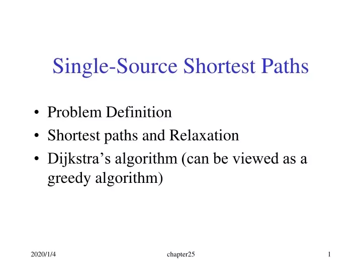
Single-Source Shortest Paths. Problem Definition Shortest paths and Relaxation Dijkstra’s algorithm (can be viewed as a greedy algorithm). Problem Definition:.

E N D
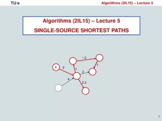
Single-Source Shortest Paths • Problem Definition • Shortest paths and Relaxation • Dijkstra’s algorithm (can be viewed as a greedy algorithm) chapter25
Problem Definition: • Real problem: A motorist wishes to find the shortest possible route from Chicago to Boston.Given a road map of the United States on which the distance between each pair of adjacent intersections is marked, how can we determine this shortest route? • Formal definition: Given a directed graph G=(V, E, W), where each edge has a weight, find a shortest path from s to v for some interesting vertices s and v. • s—source • v—destination. chapter25
B A Find a shortest path from station A to station B. -need serious thinking to get a correct algorithm. chapter25
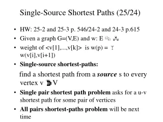
Shortest path: • The weight of path p=<v0,v1,…,vk > is the sum of the weights of its constituent edges: The cost of the shortest path from s to v is denoted as (s, v). chapter25
Negative-Weight edges: • Edge weight may be negative. • negative-weight cycles– the total weight in the cycle (circuit) is negative. • If no negative-weight cycles reachable from the source s, then for all v V, the shortest-path weight remains well defined,even if it has a negative value. • If there is a negative-weight cycle on some path from s to v, we define = - . chapter25
a b -4 h i 3 -1 2 4 3 c d 6 8 5 -8 3 5 11 g s 0 -3 e 3 f j 2 7 -6 Figure1 Negative edge weights in a directed graph.Shown within each vertex is its shortest-path weight from source s.Because vertices e and f form a negative-weight cycle reachable from s,they have shortest-path weights of - . Because vertex g is reachable from a vertex whose shortest path is - ,it,too,has a shortest-path weight of - .Vertices such as h, i ,and j are not reachable from s,and so their shortest-path weights are , even though they lie on a negative-weight cycle. chapter25
Representing shortest paths: • we maintain for each vertex vV , a predecessor [v] that is the vertex in the shortest path right before v. • With the values of , a backtracking process can give the shortest path. (We will discuss that after the algorithm is given) chapter25
Observation: (basic) • Suppose that a shortest path p from a source s to a vertex v can be decomposed into s u v for some vertex u and path p’. Then, the weight of a shortest path from s to v is We do not know what is u for v, but we know u is in V and we can try all nodes in V in O(n) time. Also, if u does not exist, the edge (s, v) is the shortest. Question: how to find (s, u), the first shortest from s to some node? chapter25
Relaxation: • The process of relaxing an edge (u,v) consists of testing whether we can improve the shortest path to v found so far by going through u and,if so,updating d[v] and [v]. • RELAX(u,v,w) • if d[v]>d[u]+w(u,v) • then d[v] d[u]+w(u,v) (based on observation) • [v] u chapter25
u v u v 2 2 5 9 5 6 RELAX(u,v) RELAX(u,v) u v u v 2 2 5 7 5 6 (a) (b) Figure2 Relaxation of an edge (u,v).The shortest-path estimate of each vertex is shown within the vertex. (a)Because d[v]>d[u]+w(u,v) prior to relaxation, the value of d[v] decreases. (b)Here, d[v] d[u]+w(u,v) before the relaxation step,so d[v] is unchanged by relaxation. chapter25
Initialization: • For each vertex v V, d[v] denotes an upper bound on the weight of a shortest path from source s to v. • d[v]– will be (s, v) after the execution of the algorithm. • initialize d[v] and [v] as follows: . • INITIALIZE-SINGLE-SOURCE(G,s) • for each vertex v V[G] • do d[v] • [v] NIL • d[s] 0 chapter25
Dijkstra’s Algorithm: • Dijkstra’s algorithm assumes that w(e)0 for each e in the graph. • maintain a set S of vertices such that • Every vertex v S, d[v]=(s, v), i.e., the shortest-path from s to v has been found. (Intial values: S=empty, d[s]=0 and d[v]=) • (a) select the vertex uV-S such that d[u]=min {d[x]|x V-S}. Set S=S{u} (b) for each node v adjacent to u doRELAX(u, v, w). • Repeat step (a) and (b) until S=V. chapter25
Continue: • DIJKSTRA(G,w,s): • INITIALIZE-SINGLE-SOURCE(G,s) • S • Q V[G] • while Q • do u EXTRACT -MIN(Q) • S S {u} • for each vertex v Adj[u] • do RELAX(u,v,w) chapter25
Implementation: • a priority queue Q stores vertices in V-S, keyed by their d[] values. • the graph G is represented by adjacency lists. chapter25
1 8 8 10 9 0 3 4 6 2 7 5 8 8 2 u v s y x (a) chapter25
u v 1 10/s 8 10 9 s 0 3 4 6 2 7 5 5/s 8 2 y x (b) (s,x) is the shortest path using one edge. It is also the shortest path from s to x. chapter25
u v 1 8/x 14/x 10 9 s 0 3 4 6 2 7 5 5/s 7/x 2 y x (c) chapter25
u v 1 8/x 13/y 10 9 s 0 3 4 6 2 7 5 5/s 7/x 2 y x (d) chapter25
u v 1 8/x 9/u 10 9 s 0 3 4 6 2 7 5 5/s 7/x 2 y x (e) chapter25
u v 1 8/x 9/u 10 9 s 0 3 4 6 2 7 5 5/s 7/x 2 y x (f) Backtracking: v-u-x-s chapter25
Backtracting code: print out the path from u to s. print (u) x=(u) while (x ≠ s) print (x) x=(x) print x chapter25
Theorem: Consider the set S at any time in the algorithm’s execution. For each vS, the path Pv is a shortest s-v path. Proof: We prove it by induction on |S|. • If |S|=1, then the theorem holds. (Because d[s]=0 and S={s}.) • Suppose that the theorem is true for |S|=k for some k>0. • Now, we grow S to size k+1 by adding the node v. chapter25
Proof: (continue) Now, we grow S to size k+1 by adding the node v. Let (u, v) be the last edge on our s-v path Pv, i.e., d[v]=d[u]+w(u, v). Consider any other path from P: s,…,x,y, …, v. (red in the Fig.) Case 1: y is the first node that is not in S and xS. Since we always select the node with the smallest value d[] in the algorithm, we have d[v]d[y]. Moreover, the length of each edge is 0. Thus, the length of Pd[y]d[v]. That is, the length of any path d[v]. y x Case 2: such a y does not exist. d[v]=d[u]+w(u, v)d[x]+w(x, v). That is, the length of any path d[v]. s u v Set S chapter25
The algorithm does not work if there are negative weight edges in the graph . u -10 2 v s 1 S->v is shorter than s->u, but it is longer than s->u->v. chapter25
Time complexity of Dijkstra’s Algorithm: • Time complexity depends on implementation of the Queue. • Method 1: Use an array to story the Queue • EXTRACT -MIN(Q) --takes O(|V|) time. • Totally, there are |V| EXTRACT -MIN(Q)’s. • time for |V| EXTRACT -MIN(Q)’s is O(|V|2). • RELAX(u,v,w) --takes O(1) time. • Totally |E| RELAX(u, v, w)’s are required. • time for |E| RELAX(u,v,w)’s is O(|E|). • Total time required is O(|V|2+|E|)=O(|V|2) • Backtracking with [] gives the shortest path in inverse order. • Method 2: The priority queue is implemented as a adaptable heap. It takes O(log n) time to do EXTRACT-MIN(Q) as well as | RELAX(u,v,w). The total running time is O(|E|log |V| ). chapter25