Development of Modern Numerical Weather Prediction

1. Development of Modern Numerical Weather Prediction

2. Vilhelm Bjerknes’ Vision • 1901 – Wanted to incorporate physics into weather forecasting • Start with complete set of initial conditions (3-D) • Solve equations using graphical methods • Initial state not sufficient for good forecasts • Did not use continuity equation to derive the initial vertical wind component (no direct measurements available) Source: Historical Essays on Meteorology 1919-1995, AMS

3. Lewis F. Richardson • About same time as Bjerknes; WWI ambulance driver • Used continuity equation to obtain initial vertical velocities, as well as the other “primitive equations” • Failed due to insufficient initial data • Solved equations by hand! • Time steps were too large – would have resulted in computational instability Source: Historical Essays on Meteorology 1919-1995, AMS

4. Further Developments • Carl-Gustaf Rossby (1939) • Showed that atmospheric longwave motion could be explained by vorticity distribution • Wave movement function of wavelength and speed of large-scale zonal flow (Rossby Waves) • Jule Charney (1949) • Developed first barotropic model • Large-scale motions approximately geostrophic and hydrostatic; no vertical motions; no vertical wind shear • Numerical prediction now realizable as soon as computers become powerful enough to run the computations Source: Historical Essays on Meteorology 1919-1995, AMS

5. First Numerical Forecast • Charney barotropic model run on ENIAC computer (1950) • Produced 500 mb height forecast • Bad forecast but looked realistic ENIAC Computer Jule Charney Source: Historical Essays on Meteorology 1919-1995, AMS

6. Operational Numerical Weather Prediction • May 6, 1955 – First regular and continuing NWP forecasts issued for U.S. • Early results worse than lab experiments • Limitations of assumptions made in the models (Quasi-geostrophic approximation) • Many storms missed; public confidence wanes • Many early problems due to bad input data from global observation networks • Barotropic model (Charney) worked best for several years • Barotropic processes mostly controlled large-scale daily motions (e.g. long waves), while baroclinic controlled short-bursts of activity (e.g. mid-latitude cyclones) Source: Historical Essays on Meteorology 1919-1995, AMS

7. The Final Major Evolution • Successful NWP using full suite of primitive equations occurred in 1966 • Original Bjerknes/Richardson vision! • Advances in computational power and improvements in input data let to acceptable forecasts • Forecasts improved almost 50% in 10-years (1955-1965) from subjective forecasts Source: Historical Essays on Meteorology 1919-1995, AMS

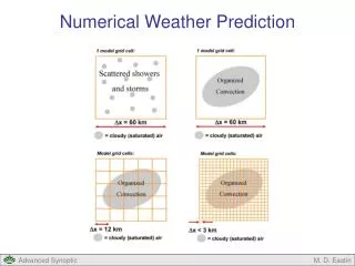
9. Types of Numerical Models • Barotropic Model • Barotropic atmosphere (constant density/temperature on pressure surface, no vertical motion) • Absolute vorticity conserved • Somewhat skillful at large-scale wave prediction

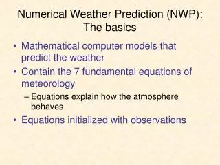
10. Types of Numerical Models • Primitive Equation Models (“Dynamical”) • The “primitive equations” are fundamental relationships that govern atmospheric motion • Equations of motion (3) (cons. of momentum) • Continuity equation (cons. of mass) • First law of thermodynamics (cons. of energy) • Moisture equation (cons. of moisture) • Equation of state • First operational baroclinic models • Use began in the mid-1960s

11. Other Models • Statistical • Forecasts based off of past events • Cannot predict extreme events • Knowledge limited to what has occurred before • Statistical-Dynamical (hybrid) • Combines some NWP output with historical statistics • Example: The SHIPS hurricane intensity model uses model fields as predictors for a statistical regression