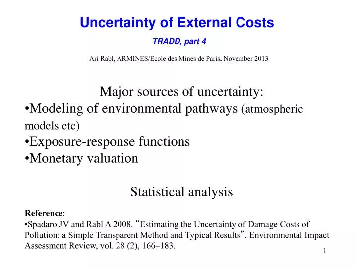
Major sources of uncertainty: Modeling of environmental pathways (atmospheric models etc )

1. Major sources of uncertainty: • Modeling of environmental pathways (atmospheric models etc) • Exposure-response functions • Monetary valuation • Statistical analysis • Reference: • Spadaro JV and Rabl A 2008. “Estimating the Uncertainty of Damage Costs of Pollution: a Simple Transparent Method and Typical Results”. Environmental Impact Assessment Review, vol. 28 (2), 166–183. Uncertainty of External CostsTRADD, part 4Ari Rabl, ARMINES/Ecole des Mines de Paris, November 2013

2. i) data uncertainty e.g. slope of a dose-response function, cost of a day of restricted activity, and deposition velocity of a pollutant; ii) model uncertainty e.g. assumptions about causal links between a pollutant and a health impact, assumptions about form of a dose-response function (e.g. with or without threshold), and choice of models for atmospheric dispersion and chemistry; iii) uncertainty about policy and ethical choices e.g. discount rate for intergenerational costs, and value of statistical life; iv) uncertainty about the future e.g. the potential for reducing crop losses by the development of more resistant species; v) idiosyncrasies of the analyst e.g. interpretation of ambiguous or incomplete information, and human error. The difficulties begin with trying to prepare this list: the distinction between these sources is not always clear. Sources of uncertainty

3. For data and model uncertainties: analysis by statistical methods, combining the component uncertainties over the steps of the impact pathway, to obtain formal confidence intervals around a central estimate. For ethical choice, uncertainty about the future, and subjective choices of the analyst: sensitivity analysis, indicating how the results depend on these choices and on the scenarios for the future. For human error: be careful and guard against overconfidence. Appropriate analysis

4. Quantifying the sources of uncertainty in this field is problematic because of a general lack of information. Usually one has to fall back on subjective judgment, preferably by the experts of the respective disciplines. The uncertainties due to strategic choices of the analyst, e.g. which dose-response functions to include, are difficult to take into account in a formal uncertainty analysis.  the comprehensive uncertainties can be much larger than the ones that have been quantified (uncertainties due to data and parameters). Difficulties

5. Don’t confuse uncertainty and variability of impacts! Both can cause estimates to change, but in very different ways and for totally different reasons: Uncertainty: insufficient knowledge at the present time, future estimates may be different when we know more. Variability: damage cost can vary with the type of source (where, ground level or tall stacks, …). Damage cost per kWh are proportional to the emissions and vary with the technologies used. These variations are independent of the uncertainties. Uncertainty  variability

6. Variability of damage with site An example of dependence on site and on height of source for a primary pollutant: damage D from SO2 emissions with linear ER function, for five sites in France, in units of Duni for uniform world model Eq.10 with  = 105 persons/km2 (the nearest big city, 25 to 50 km away, is indicated in parentheses). The scale on the right indicates YOLL/yr (years of life lost) by acute mortality from a plant with emission 1000 ton/yr. Plume rise for typical power plant conditions is accounted for.

7. Damage costs of fossil power plants (€/kg of ExternE [2008]). Also shown are the damage costs for coal and oil plants in France during the mid nineties. For comparison: market price in France was about 7 €cents/kWh during the mid nineties, and 11 €cents/kWh in 2011. Variability of damage cost, due to changed emissions

8. Probability distributions of parameter values The most important characteristics are the mean  and the standard deviation  Example: the frequent case of a normal (=gaussian) distribution with  = 0 and  = 1 Confidence intervals 68% [ - ,  + ] 95% [ - 2,  + 2] 68% Confidence interval

9. For a sum the standard deviation , and for a product the standard geometric deviation g, can be calculated exactly, regardless how wide the distributions of the individual terms. Furthermore, the entire distribution is often approximately normal (for sums) or lognormal (for products). • Explicit closed form solution! • But for general functions y = f(x1, x2, …, xn) a closed form solution can be obtained only in the limit of small uncertainties (narrow distributions) Combination of errors for a general function of terms That is not appropriate for the large uncertainties of external costs. Generalsolution viaMonte Carlo calculation, i.e. perform a very large number of numerical simulations, each calculating the result y for a specific choice of {x1, x2, … xn}, and look at the resulting distribution of the y.

10. Combination of errors for a sum of terms Ify = x1 + x2 + … + xn is a sum of uncorrelated random variables xi, each with mean mi and standard deviation si, the uncertainty distribution of y has mean  = 1 + 2 + … + n, and standard deviation sy given by y2 = 12 + 22 + … + n2. That result is general, but for confidence intervals one also needs the distribution. In practice the distribution of y is often close to normal even for very small n if the individual distributions (especially those with large widths) are not too far from normal. Justified by central limit theorem of statistics: In the limit n, the distribution of y approaches a normal distribution, even if the distributions of the individual xi are not normal.

11. Combination of errors for a product of terms If y = x1 x2 … xn, the log of y is a sum ln(y) = ln(x1) + ln(x2) + … + ln(xn). Let the xi be uncorrelated random variables with probability distributions pi(xi). Define the geometric mean gi of xi by Then the geometric mean gy of y is given by and it is equal to gy = g1g2 … gn

12. Combination of errors for a product of terms, cont’d Now define the geometric standard deviation gi of xi by Then the geometric standard deviation gy of y is given by [ln(gy)]2 = [ln(g1)]2 + [ln(g2)]2 + … + [ln(gn)]2 That result is general, but for confidence intervals one also needs the distribution. In practice the distribution of ln(y) is often approximately normal, if the distributions of the individual ln(xi) are not too far from normal. A variable whose log has a normal distribution is called lognormal. The distribution of a product is often approximately lognormal.

13. The lognormal distribution To get the lognormal from the normal distribution Change variable u = ln(x). Then du = dx/x and normalization integral becomes which allows interpreting the function as the probability density of a new distribution between 0 and . This is the lognormal distribution, with  = ln(g) or g= exp()= geometric mean and  = ln(g) or g= exp() = geometric standard deviation

14. g 68% confid. interval The lognormal distribution, cont’d The lognormal distribution is asymmetric, with a long tail and its mean is larger than its median. Its median is equal to g. p(x) Example, with g = 1 and g = 2 x When plotted vsln(x) it looks just like an ordinary normal. For confidence intervals, note that 68% of the distribution is in the interval [g/ g, gg] and 95% of the distribution is in the interval [g/ g2, gg2] .

15. Probability density of lognormal distribution with g = 1 and g = 3. Mean  = 1.83. The arrows indicate the 68% confidence interval (1g interval). p(x) Lognormal Distribution, cont’d x

16. Estimation of uncertainties with Uniform World Model the damage costC per quantity Q of pollutant is a product C = P sER Q/vdep . • P = “price” = unit cost of endpoint (e.g. value of a life year) • sER = slope of exposure-response function • = regional average receptor density (with radius of about 1000 km) vdep = depletion velocity These factors are uncorrelated  can use simple solution with g For a finer analysis each of the factors p, sER and vdep can be broken up into separate factors to account for their respective uncertainty sources. Comparison of UWM with detailed site specific calculations for about a hundred installations in many countries of Europe, as well as China, Thailand and Brazil: UWM is so close to the average that it can be recommended fortypical damage costs for emissions from tall stacks (>~ 50 m); for specific sites the agreement is usually within a factor of two to three. Note: typical values = average over emission sites, equivalent to averaging over receptor distributions   becomes uniform.

17. Calculation is approximately multiplicative •  distribution of errors is approximately lognormal • (unless the contributions with the largest g have a distribution that is very different from lognormal) • characterized by geometric standard deviation g • Multiplicative confidence intervals aboutgeometric mean g(smaller than ordinary mean ) • 68% between g/g and gg • 95% between g/g2 and gg2 Confidence intervals

18. Uncertainty of the components, cont’d Example of lognormal distribution for monetary valuation: “value of statistical life”, in £1990, in 78 studies reviewed by Ives, Kemp and Thieme [1993], histogram and lognormal fit. Approximately lognormal g = 1.5 M£ g = 3.4

19. Uncertainty of the components For Dispersion: deposition velocities. example: Distribution and lognormal fit of data points in the review of Sehmel [1980], for dry deposition velocity [in cm/s] of SO2 over different surfaces. Approximately lognormal

20. Uncertainty of the components, cont’d How to estimate an approximate equivalent geometric standard deviation g when one only knows mean  and ordinary standard deviations  Assume that the one-standard deviation (68% probability) interval [- ,  + ] corresponds to the interval [g/g, gg] of the lognormal distribution  Many studies (e.g. epidemiology) report their errors as 95% confidence intervals, corresponding to two ordinary standard deviations,[- 2 ,  + 2 ] . In that case use

21. Uncertainty, with UWM C = P sER Q/vdep [ln(gC)]2 = [ln(gp)]2 + [ln(gsER)]2 + [ln(g)] + [ln(gQ)] + [ln(gvdep)] 2 Note: Only the largest errors make significant contribution

22. Uncertainty of mortality cost, more detail [ln(gy)]2 = [ln(g1)]2 + [ln(g2)]2 + … + [ln(gn)]2 Note: Only the largest errors make significant contribution

23. Monte Carlo  simplified analysis For damage costs the two approaches are complementary

24. Presentation of uncertainty Damage costs for LCA applications in EU27, €/kg h = stack height

25. (these values are for LCA applications in Europe) The changes are within the published uncertainty intervals Evolution of damage cost estimates(due to scientific progress, especially epidemiology and monetary valuation)

26. Effect of uncertainties • depends on specifics of each decision, e.g. • choice of technology (e.g. coal or nuclear) • optimal pollution control (e.g. mg/m3 of SO2 in smoke stack) • level of pollution tax (e.g. €/tonne of SO2) • replacement of old dirty technologies (e.g. old cars) • choice of site (e.g. rural or urban) • green accounting • Key question: • What is life cycle cost penalty to society if decision based on erroneous damage estimate? • discrete choices: no effect if uncertainty does not change ranking • continuous choices: sensitivity to uncertainty is small near optimum

27. Effect of uncertainties, discrete choices Example where tighter regulation is justified: new directive [EC 2000] for waste incineration Example where tighter regulation is not justified: reduced PM emission limits for cement kilns

28. Effect of uncertainties, continuous choices, cont’d Cost penalty ratio R = The cost penalty ratio R versus the error x = Dtrue/Dest in the damage cost estimate for several countries, selected to show extremes as well as intermediate curves. The labels are placed in the same order as the curves. Dashed lines correspond to the extrapolated regions of the cost curves. Similar results for NOx and CO2

29. The uncertainties of damage costs are large, • typically geometric standard deviations g around 3 to 5 • g around 3 for primary pollutants PM, NOx,SO2; • somewhat larger for secondary pollutants (especially O3) than for primary pollutants; • g around 4 for toxic metals (As, Cd, Cr, Hg, Ni and Pb); • g around 5 for greenhouse gases. Conclusion on Uncertainties

30. Effect of uncertainties Some people think that the uncertainties of ExternE estimates are too large to be useful However: 1) Better 1/3 x to 3 x than 0 to  2) What matters is not the uncertainty itself, but the social cost of a wrong choice: a) Without cost estimates such costs can be very large, but with ExternE they can be remarkably small in many if not most cases. b) For many yes/no choices the uncertainty is small enough not to affect the answer. 3) Uncertainties can be reduced by a) research and b) guidelines by decision makers on monetary values

31. Extra social cost due to errors Without cost estimates such costs can be very large, but with ExternE they can be remarkably small in many if not most cases. Example: extra social cost (relative to optimum with perfect information) forNOx abatement: less than 15% within confidence interval, but gets very large for much larger errors: Ctrue = true damage cost Cest= estimated damage cost Thanks to ExternE one can avoid very costly mistakes.