Non-linear regression

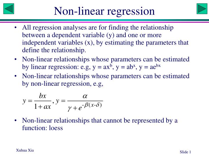
1. Non-linear regression • All regression analyses are for finding the relationship between a dependent variable (y) and one or more independent variables (x), by estimating the parameters that define the relationship. • Non-linear relationships whose parameters can be estimated by linear regression: e.g, y = axb, y = abx, y = aebx • Non-linear relationships whose parameters can be estimated by non-linear regression, e.g, • Non-linear relationships that cannot be represented by a function: loess

2. Growth curve of E. coli • A researcher wishes to estimate the growth curve of E. coli. He put a very small number of E. coli cells into a large flask with rich growth medium, and take samples every half an hour to estimate the density (n/L). • 14 data points over 7 hours were obtained. • What is the instantaneous rate of growth (r). What is the initial density (N0)? • As the flask is very large, he assumed that the growth should be exponential, i.e., y = a·ebx (Which parameter correspond to r and which to N0?)

3. SAS Program /* Fictitious data */ data Ecoli; Input Density @@; Time = _N_; lnD = log(Density); datalines; 20.023 39.833 80.571 161.102 317.923 635.672 1284.544 2569.430 5082.654 10220.777 20673.873 40591.439 81374.642 163963.873 ; proc reg; var Density lnD Time; model lnD = Time; plot Density*Time/ symbol='.'; plot lnD*Time/ symbol='.'; run; This statement is necessary, otherwise Density will be an unknown variable for the reg procedure and the plot statement will fail. Run, and ask students to compute parameters a and b from regression output. What is the initial density?

4. Body weight of wild elephant • A researcher wishes to estimate the body weight of wild elephants. • He measured the body weight of 13 captured elephants of different sizes as well as a number of predictor variables, such as leg length, trunk length, etc. Through stepwise regression, he found that the inter-leg distance (shown in figiure) is the best predictor of body weight. • He learned from his former biology professor that the allometric law governing the body weight (W) and the length of a body part (L) states thatW = aLb • Use linear regression to find parameters a and b.

5. SAS Program /*Fitcitious data */ data Elephant; Input L W @@; lnL = log(L); lnW = log(W); datalines; 0.3 1.657 0.4 2.500 0.5 4.680 0.6 7.075 0.7 10.070 0.8 11.988 0.9 14.836 1 18.318 1.1 23.496 1.2 27.897 1.3 36.796 1.4 44.611 1.5 50.183 ; proc reg; var L W lnL lnW; model lnW = lnL; plot W*L/ symbol='.'; plot lnW*lnL/ symbol='.'; run; Run and ask students to calculate the parameters a and b.

6. DNA and protein gel electrophoresis • How to estimate the molecular mass of a protein? • A ladder: proteins with known molecular mass • Deriving a calibration curve relating molecular mass (M) to migration distance (D): D = F(M) • Measure D and obtain M • The calibration curve is obtained by fitting a regression model

7. Protein molecular mass • The equation appears to describe the relationship between D and M quite well. This relationship is better than some published relationships, e.g., D = a – b ln(M) • The data are my measurement of D and M for a subset of secreted proteins from the gastric pathogen Helicobacter pylori (Bumann et al., 2002). • Write a SAS program to use the data to find parameters a and b Bumann, D., Aksu, S., Wendland, M., Janek, K., Zimny-Arndt, U., Sabarth, N., Meyer, T.F., and Jungblut, P.R., 2002, Proteome analysis of secreted proteins of the gastric pathogen Helicobacter pylori. Infect. Immun. 70: 3396-3403.

8. Area and Radius What is the functional relationship between the area and the radius?

9. Toxicity study: pesticide What transformation to use?

10. Probit and probit transformation • Probit has two names/definitions, both associated with standard normal distribution: • the inverse cumulative distribution function (CDF) • quantile function • CDF is denoted (z), which is a continuous, monotone increasing sigmoid function in the range of (0,1), e.g.,(z) = p(-1.96) = 0.025 = 1 - (1.96) • The probit function gives the 'inverse' computation, formally denoted -1(p), i.e.,probit(p) = -1(p) probit(0.025) = -1.96 = -probit(0.975) • [probit(p)] = p, and probit[(z)] = z.

11. SAS program Data Pesticide; Input Dosage Percent @@; NuProbit = probit(Percent/100); Cards; 27 0.90 28 1.39 31 2.40 31 2.49 35 6.42 36 7.78 37 9.16 38 10.21 38 11.71 40 16.24 41 16.90 43 22.94 44 27.35 44 27.45 44 28.14 45 28.97 45 29.96 45 30.50 46 34.30 46 35.39 46 35.65 47 37.55 47 38.46 48 40.97 49 44.37 49 45.71 49 46.66 49 47.38 50 49.86 50 52.26 51 55.12 51 56.12 52 57.68 52 59.99 52 60.30 53 60.51 53 61.82 53 62.00 53 62.92 54 66.06 54 67.14 55 70.58 55 71.57 56 74.11 56 74.12 57 76.77 57 77.01 58 78.56 58 79.01 59 83.53 60 83.96 60 84.40 61 87.95 62 88.74 63 91.13 64 92.64 64 92.67 66 95.49 68 97.00 69 97.15 ; Procreg; Model Percent = Dosage / R CLM alpha = 0.01 CLI; Plot Percent*Dosage / symbol = '.'; Model NuProbit = Dosage / R CLM alpha = 0.01 CLI; Plot NuProbit*Dosage / symbol = '.'; run; Why divide Percent by 100? Run and explain CLM: CL of mean CLI: CL of individual observation Graphic contrast between the original and the transformed DV

12. Non-linear regression • In rapidly replicating unicellular eukaryotes such as the yeast, highly expressed intron-containing genes requires more efficient splicing sites than lowly expressed genes. • Natural selection will operate on the mutations at the slicing sites to optimize splicing efficiency. • Designate splicing efficiency as SE and gene expression as GE. • Certain biochemical reasoning suggests that SE and GE will follow the following relationships:

13. Guess initial values When GE=0 then SE = , so   0.4 When GE increases from 2 to 8, SE increases from 0.47 to 0.75, so   (0.75-0.47)/(8-2)  0.047 With   0.4 and   0.047, then SE for GE = 12 should be 0.4+0.04712 = 0.96, but the actual SE is only about 0.77. This must be due to the quadratic term GE2, i.e., (0.77 - 0.96) =  122, so   - 0.002

14. A few more twists The continuity condition requires that The smoothness condition requires that The two conditions implies that

15. SAS program /* Fictitious data */ data Intron; input SE GE @@; datalines; .46 1 .47 2 .57 3 .61 4 .62 5 .68 6 .69 7 .78 8 .70 9 .74 10 .77 11 .78 12 .74 13 .80 13 .80 15 .78 16 ; title 'Quadratic Model with Plateau'; proc nlin data=Intron; parms alpha=.4 beta=.047 gamma=-.002; GE0 = -.5*beta / gamma; if (GE < GE0) then Y = alpha + beta*GE + gamma*GE*GE; else Y = alpha + beta*GE0 + gamma*GE0*GE0; model SE = Y; if _obs_ =1 and _iter_ =. then do; plateau =alpha + beta*GE0 + gamma*GE0*GE0; put / GE0= plateau= ; end; output out=b predicted=SEp; run; Initial guestimates A conditional statement needed to model the two segments Write out GE0 and plateau (which could be computed from the estimated , , and . However, the output of these parameters contain rounding errors. computes predicted values for plotting and saves them to data set b Run and explain

16. Plot proc sgplot data=b noautolegend; yaxis label='Observed or Predicted'; refline 0.7775 / axis=y label="Plateau" labelpos=min; refline 12.7476 / axis=x label="GE0" labelpos=min; scatter y=SE x=GE; series y=SEp x=GE; run;

17. Fitting another function /* Fictitious data */ data Intron; input SE GE @@; datalines; .46 1 .47 2 .57 3 .61 4 .62 5 .68 6 .69 7 .78 8 .70 9 .74 10 .77 11 .78 12 .74 13 .80 13 .80 15 .78 16 ; title 'Quadratic Model with Plateau'; proc nlin data=Intron; parms alpha=.4 beta=.8 gamma=1; model SE = (alpha+beta*GE)/(1+gamma*GE); output out=b predicted=SEp; run; proc sgplot data=b noautolegend; yaxis label='Observed or Predicted'; scatter y=SE x=GE; series y=SEp x=GE; run; Run and explain the output

18. Plot output

19. Robust regression • LOWESS: robust local regression between Y and X, with linear fitting • LOESS: robust local regression between Y and one or more Xs, with linear or quadratic fitting • Used with relations that cannot be expressed in functional forms • SAS: proc loess • Data: • Data set 1: monthly averaged atmospheric pressure differences between Easter Island and Darwin, Australia for a period of 168 months (NIST, 1998), suspected to exhibit 12-month (annual), 42-month (El Nino), and 25-month (Southern Oscillation) cycles (From Robert Cohen of SAS Institute) • Data set 2: Two-channel microarray data. Background correction and two-channel loess normalization (from Wudu).

22. Step 1: characterize the most obvious trend. data ENSO; input Pressure @@; Month=_N_; datalines; 12.9 11.3 10.6 11.2 10.9 7.5 7.7 11.7 12.9 14.3 10.9 13.7 17.1 14.0 15.3 8.5 5.7 5.5 7.6 8.6 7.3 7.6 12.7 11.0 12.7 12.9 13.0 10.9 10.4 10.2 8.0 10.9 13.6 10.5 9.2 12.4 12.7 13.3 10.1 7.8 4.8 3.0 2.5 6.3 9.7 11.6 8.6 12.4 10.5 13.3 10.4 8.1 3.7 10.7 5.1 10.4 10.9 11.7 11.4 13.7 14.1 14.0 12.5 6.3 9.6 11.7 5.0 10.8 12.7 10.8 11.8 12.6 15.7 12.6 14.8 7.8 7.1 11.2 8.1 6.4 5.2 12.0 10.2 12.7 10.2 14.7 12.2 7.1 5.7 6.7 3.9 8.5 8.3 10.8 16.7 12.6 12.5 12.5 9.8 7.2 4.1 10.6 10.1 10.1 11.9 13.6 16.3 17.6 15.5 16.0 15.2 11.2 14.3 14.5 8.5 12.0 12.7 11.3 14.5 15.1 10.4 11.5 13.4 7.5 0.6 0.3 5.5 5.0 4.6 8.2 9.9 9.2 12.5 10.9 9.9 8.9 7.6 9.5 8.4 10.7 13.6 13.7 13.7 16.5 16.8 17.1 15.4 9.5 6.1 10.1 9.3 5.3 11.2 16.6 15.6 12.0 11.5 8.6 13.8 8.7 8.6 8.6 8.7 12.8 13.2 14.0 13.4 14.8 ; ods output OutputStatistics=ENSOstats FitSummary=ENSOsummary; proc loess data=ENSO; model Pressure=Month / CLM smooth = 0.02 to 0.2 by 0.01 dfmethod=exact; run; symbol1 c=black i=join value=dot; symbol2 c=black i=join value=none; proc gplot data=ENSOstats; by SmoothingParameter; plot (DepVar Pred)*Month/overlay; run; The output data ENSOstats contains variables: SoothingParameter, Month, DepVar, Pred, etc. Three criteria for choosing the smooth parameter: GCV: generalized cross-validation (Craven and Wahba 1979) AIC: Akaike information criterion (Akaike 1973) AICC1: bias-corrected AIC (JUrvich and Simonoff 1988)

23. Summary output: kd Tree, linear max(1, n*s/5) int(n*s), where n is ‘N. Fitting Points’ and s is ‘Smotthing Param.’

24. More on Output

26. proc loess data=ENSO; model Pressure=Month / smooth = 0.01 to 0.2 by 0.01 dfmethod=exact degree = 2; run; SmoothingParameter=0.05 Pressure 18 17 16 15 14 13 12 11 10 9 8 7 6 5 4 3 2 1 0 0 10 20 30 40 50 60 70 80 90 100 110 120 130 140 150 160 170 Month

27. 99% Confidence limits ods output OutputStatistics=ENSOstats FitSummary=ENSOsummary; proc loess data=ENSO; model Pressure=Month / r CLM smooth = 0.05 alpha=0.01 dfmethod=exact; run; symbol1 c=black i=none value=dot; symbol2 c=black i=join value=none; symbol3 c=red i=join value=none; symbol4 c=red i=join value=none; proc gplot data=ENSOstats; format DepVar 4.0; plot (DepVar Pred UpperCl LowerCL)*Month/ overlay hminor = 0 vminor = 0 vaxis = axis1 frame; run;

28. 99% confidence limits 20 16 12 Pressure 8 4 0 0 10 20 30 40 50 60 70 80 90 100 110 120 130 140 150 160 170 Month

29. Step 2: Characterize other trends • /* modify data set ENSO to filter out the 12-month cycle */ • data ENSO(drop=pi); • set ENSO; • pi = 4 * atan (1); /* or pi = 3.1415926 */ • cos1 = cos(2*pi*Month/12); • sin1 = sin(2*pi*Month/12); • proc reg data=ENSO; • model Pressure = cos1 sin1; • output out=ENSO1 r=FilteredPressure; • run; • proc print data=ENSO1; • var Month Pressure FilteredPressure; • run; • ods output OutputStatistics=ENSO1stats; • proc loess data=ENSO1; • model FilteredPressure=Month/ • smooth = 0.12; • run; • proc gplot data=ENSO1stats; • plot (DepVar Pred)*Month/overlay; • run; r: residual, i.e., what is left after the monthly cycle has been removed.

30. Cos1 and Sin1

31. Filtered Pressure

32. ~42-month cycle 7 6 5 4 3 2 1 0 Residual -1 -2 -3 -4 -5 -6 -7 -8 0 10 20 30 40 50 60 70 80 90 100 110 120 130 140 150 160 170 Month

33. Any other trend? /* modify data set ENSO to filter out the 12-month cycle */ data ENSO(drop=pi); set ENSO; pi = 4 * atan (1); cos1 = cos(2*pi*Month/12); sin1 = sin(2*pi*Month/12); cos2 = cos(2*pi*Month/42); sin2 = sin(2*pi*Month/42); proc reg data=ENSO; model Pressure = cos1 sin1 cos2 sin2; output out=ENSO1 r=FilteredPressure; run; proc print data=ENSO1; var Month Pressure FilteredPressure; run; ods output OutputStatistics=ENSO1stats; proc loess data=ENSO1; model FilteredPressure=Month/ smooth = 0.12; run; proc gplot data=ENSO1stats; plot (DepVar Pred)*Month/overlay; run;

34. ~25-month cycle 6 5 4 3 2 1 0 Residual -1 -2 -3 -4 -5 -6 -7 0 10 20 30 40 50 60 70 80 90 100 110 120 130 140 150 160 170 Month

35. Microarray • Diagnosis • Signature genes • Gene regulation pathway Avian coronavirus Bovine coronavirus

36. Spotted cDNA Microarray cDNA “B” Cy3 labeled cDNA “A” Cy5 labeled + Laser 1 Laser 2 Scanning Hybridization DNA molecules are immobilized by high-speed robots on a solid surface such as glass. + Analysis Image Capture

37. Microarray Data

38. Basic Microarray Data Analysis • Basic information • Channel 1 background and foreground intensity: B1, F1 • Channel 2 background and foreground intensity: B2, F2 • Because two-channel microarray typically use the red and green dye for the two channels, we have: Rb, Rf, Gb, Gf • Background correction • Within-slide normalization • Identification of differentiallyexpressed genes • Expectation of M is zero. • A gene is overexpressed (or underexpressed) if its M is significantly greater (or smaller) than 0

39. Routine analysis ODS GRAPHICS / ANTIALIASMAX=5800; Data WuduPGF7; Input X Y Ch1I Ch1B Ch2I Ch2B; R=Ch1I - Ch1B; G=Ch2I - Ch2B; if R>0 and G>0 then do; M=log2(R/G); A=log2(R*G)/2; end; else do; M=.; A=.; end; cards; 2280 8520 469.22876 166.962967 231.892853 54.888889 2510 8500 443.9776 116.055557 295.28302 73.981483 .. ; proc sgplot; scatter x=A y=M ; run;

40. MA plot

41. Microarray data: Background correction /*partial data from slide PGF7*/ Data WuduPGF7; Input X Y Ch1I Ch1B Ch2I Ch2B; cards; 2280 8520 469.22876 166.962967 231.892853 54.888889 2510 8500 443.9776 116.055557 295.28302 73.981483 2750 8500 421.165527 133.40741 227.327103 74.953705 2990 8510 401.165405 151.361115 223.877365 53.722221 ... ; proc g3d; scatter X*Y=Ch1B; run; proc loess data=WuduPGF7; model Ch1B=X Y/smooth=0.01 to 0.04 by 0.01 dfmethod=exact degree=2; run; Run the WuduPGFA.sas file

42. Two different kinds of CLM ods output OutputStatistics=StatOut FitSummary=OutSummary; proc loess data=WuduPGF7; model M=A / r CLM smooth = 0.09 alpha=0.01 dfmethod=exact; run; symbol1 c=black i=none value=dot; symbol2 c=black i=join value=none; symbol3 c=red i=join value=none; symbol4 c=red i=join value=none; proc sort data=StatOut out = StatOut2; by A; run; proc gplot data=StatOut2; format DepVar 4.0; plot (DepVar Pred UpperCl LowerCL)*A/ overlay; run; proc reg data=StatOut; model Residual=A / R CLM alpha = 0.01 CLI ; plot Residual *A / pred ; run;

43. CLM of the mean

44. CLM of the observations

45. Channel-1 background: PGF Slide 7

46. Channel-2 background: PGF Slide 7

47. Channel-1 background: 1720p Slide 1

48. Channel-2 background: 1720p Slide 1

49. Summary output Which smoothing parameter is the best?

50. Fit background surface data PredGrid; do Y = 8320 to 26230 by 230; do X = 2220 to 20250 by 230; output; end; end; ods output ScoreResults=Ch1Bscore; proc loess data=WuduPGF7; model Ch1B=X Y/smooth=0.02 dfmethod=exact; score data=PredGrid; run; proc g3d data=Ch1Bscore; format X f4.0; format Y f4.0; format p_Ch1B f4.1; plot X*Y=p_Ch1B/ tilt=60 rotate=80; run;