Download

1 / 27
280 likes | 515 Views
Item Parameter Estimation: Does WinBUGS Do Better Than BILOG-MG?. Bayesian Statistics, Fall 2009 Chunyan Liu & James Gambrell. Introduction. 3 Parameter IRT Model Assigns each item a logistic function with a variable lower asymptote. Purpose.

E N D
Item Parameter Estimation: Does WinBUGS Do Better Than BILOG-MG? Bayesian Statistics, Fall 2009 Chunyan Liu & James Gambrell
Introduction • 3 Parameter IRT Model • Assigns each item a logistic function with a variable lower asymptote.
Purpose • Compare BILOG-MG and WinBUGS estimation of item parameters under the 3 parameter logistic (3PL) IRT model • Investigate the effect of sample size on the estimation of item parameters
BILOG – MG (Mislevy & Bock 1985) • Propriety software • Uses unknown estimation shortcuts • Sometimes gives poor results • “Black Box” program • Very fast estimation • Provides only point estimates and standard errors for model parameters • Estimation method • Marginal Maximum Likelihood • Expectation-Maximization algorithm (Bock and Aitkin, 1981)
WinBUGS • More open-source (related to OpenBugs) • More widely studied • Might give more robust results • Much more flexible • Provides full posterior densities for model parameters • More output to evaluate convergence • Very slow estimation!
Literature Review • Most researchers have used custom-built MCMC samplers using Metropolis-Hastings- within-Gibbs algorithm • as recommended by Cowles, 1996! • Patz and Junker (1999a & b) • Wrote MCMC sampler in S plus • Found that their sampler produced estimates identical to BILOG for the 2PL model, but had some trouble with 3PL models. • Found MCMC was superior at handling missing data.
Literature Review • Jones and Nediak (2000) • Developed “commercial grade” sampler in C++ • Improved the Patz and Junker algoritm • Compared MCMC results to BILOG using both real and simulated data • Found that item parameters varied substantially, but the ICCs described were close according to the Hellinger deviance criterion • MCMC and BILOG were similar for real data • MCMC was superior for simulated data • Note that MCMC provides much more diagnostic out to assess convergence problems
Literature Review • Proctor, Teo, Hou, and Hsieh (2005 project for this class!) • Compared BILOG to WinBUGS • Fit a 2PL model • Only simulated a single replication • Did not use deviance or RMSE to assess error
Data • Test: 36-item multiple choice • Item parameters (a, b and c) come from Chapter 6 of Equating, Scaling and Linking (Kolen and Brennan) • Treated as true item parameters (See Appendix) • Item responses simulated using 3PL model a – slope b – difficulty c – guessing – examinee ability
Methods • N(N=200, 500, 1000, 2000) θ values were generated from N(0,1) distribution. • N item responses were simulated based on the θ’s generated in step 1 and the true item parameters using the 3PL model. • Item parameters (a, b, c for the 36 items) were estimated using BILOG-MG based on the N item responses. • Item parameters (a, b, c for the 36 items) were estimated using WinBUGS based on the N item responses using the same prior as specified by BILOG-MG. • Repeat steps two and four 100 times. For each item, we have 100 estimated parameter sets from both programs
Priors • a[i] ~ dlnorm(0, 4) • b[i] ~ dnorm(0, 0.25) • c[i] ~ dbeta(5,17) • Same priors used in BILOG and WinBUGS
Criterion-Root Mean Square Error (RMSE) • For each item, we computed the RMSE for a, b, and c using the same formula where and Here could be , , or and x could be the parameter of a, b or c
Results 1. Deciding the number of Burn-in Iterations- History Plots
Results-cont. 1. Deciding the number of Burn-in Iterations- Autocorrelation and BGR plots
Results-cont. 1. Deciding the number of Burn-in Iterations- Statistics node mean sd MC error 2.5% median 97.5% start sample a[1] 0.899 0.1011 0.004938 0.7117 0.8949 1.107 2501 3500 a[2] 1.339 0.1159 0.004132 1.125 1.333 1.58 2501 3500 a[3] 0.7308 0.111 0.005769 0.551 0.717 0.9893 2501 3500 a[4] 2.012 0.2712 0.009897 1.531 1.996 2.59 2501 3500 a[5] 1.766 0.2202 0.009585 1.394 1.745 2.243 2501 3500 b[1] -1.706 0.2944 0.01793 -2.253 -1.717 -1.1 2501 3500 b[2] -0.4277 0.1167 0.005916 -0.6571 -0.428 -0.1857 2501 3500 b[3] -0.7499 0.3967 0.01586 -1.409 -0.7994 0.1348 2501 3500 b[4] 0.4324 0.09295 0.004443 0.2363 0.4384 0.6008 2501 3500 b[5] -0.05619 0.122 0.006737 -0.3127 -0.05246 0.1657 2501 3500 c[1] 0.2458 0.088 0.004718 0.09253 0.2415 0.4362 2501 3500 c[2] 0.1403 0.04745 0.002158 0.05368 0.139 0.2361 2501 3500 c[3] 0.2538 0.09285 0.005864 0.09991 0.243 0.4557 2501 3500 c[4] 0.2669 0.035 0.001491 0.1911 0.2693 0.3282 2501 3500 c[5] 0.2588 0.05029 0.002589 0.1526 0.261 0.35 2501 3500
Results-cont. 1. Running conditions for WinBUGS • Adaptive phase: 1000 iterations • Burn-in: 1500 iterations • For computing the Statistics: 3500 iterations • Using 1 chain • Using bugs( ) function to run WinBUGS through R • Need BRugs and R2WinBUGS packages
Results-cont. 2. Effect of Sample Size
Results-cont. BILOG-MG vs. WinBUGS – a parameter
Results-cont. BILOG-MG vs. WinBUGS - b parameter
Results-cont. BILOG-MG vs. WinBUGS - c parameter
Discussion & Conclusions • Larger sample size decreased RMSE for all parameters under both programs. • For N=200, there was a significant convergence problem for BILOG-MG. No problem with WinBUGS.
Discussion & Conclusions-cont. • Slope parameter “a” • WinBUGS was superior to BILOG when N = 500 or less • More accurately estimated for items without extreme a or b parameters by both programs. • Difficulty parameter “b” • BILOG was superior to WinBUGs when N = 500 or less • Both programs had larger error for items either too difficult or too easy • Guessing parameter “c” • WinBUGs was superior to BILOG at all sample sizes, but especially at N = 1,000 or less • More accurately estimated for difficult items by both programs. • Both programs had larger error for items with shallow slopes.
Limitations • Only one chain is used in the simulation study. • Some of the MC errors are not less than 1/20 of the standard deviation, could use more iterations in MCMC sampler • Simulated data • Conforms to the 3PL model much more closely than real data would • No missing responses • No omit problems • Fewer low scores
WinBUGS code for running 3PL model 3PL; { for (i in 1:N) { for (j in 1:n) { e[i,j]<-exp(a[j]*(theta[i]-b[j])) p[i,j] <- c[j]+(1-c[j])*(e[i,j]/(1+e[i,j])) resp[i,j] ~ dbern(p[i,j]) } theta[i] ~ dnorm(0,1) } for (i in 1:n) { a[i] ~ dlnorm(0, 4) b[i] ~ dnorm(0, 0.25) c[i] ~ dbeta(5,17) } }
Acknowledgement • Professor Katie Cowles