ABSTRACT

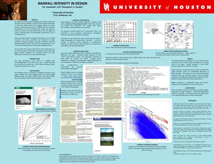
1. RAINFALL INTENSITY IN DESIGN T.G. Cleveland1, D.B. Thompson2, S. Sunder3 1 University of Houston 2 R.O. Anderson, Inc. ABSTRACT An empirical, dimensionless-hyetograph that relates depth and duration, and thus whether a storm is front loaded, back loaded, or uniformly loaded, based on 92 gaging stations for storms known to have produced runoff is available for Texas. Statistical characteristics of storm interevent time, depth, and duration, based on analysis of hourly rainfall data for 533 rain gages are used to “dimensionalize” this hyetograph and produce a set of simulated storms. These simulated storms are analyzed to generate a set of rainfall intensities, and these intensities are compared to global maximum observed rainfalls, intensities estimated using the National Weather Service TP-40, and HY-35 publications, and a current Texas Department of Transportation design equation. The simulated storms agree well with the other methods for rare (i.e. 90-th percentile and above) occurrences and lie within the global maxima envelope. The simulated results are quite different for common (i.e. 50-th percentile) events. EMPIRICAL HYETOGRAPHS Sether-Williams and others (2004) analyzed 92 stations, 1507 storms, known to have produced runoff. Each storm duration was divided into 4-quartiles. The quartile with largest accumulation of rainfall defines “storm quartile.” The observed rainfall collected into 2.5-percentile “bins” and smoothed to force monotonic dimensionless hyetographs. Result is empirical-dimensionless-hyetograph. Subsequent to that report, the authors noted that the slopes of these hyetographs are dimensionless “intensity”. Used that concept to generate various collections of dimensionless intensity, but need a way to dimensionalize for comparison to actual data or for practical application. L-MOMENT TABULATIONS Used to dimensionalize the empirical hyetograph HARRIS COUNTY RAINGAGE STATIONS Four (4) stations used in example calculations. Tabular values of L-moments (and equations) are shown in figure below. INTENSITY SIMULATION Asquith and others (2006), analyzed 774 stations in New Mexico, Oklahoma, and Texas. Generated depth quantiles for each “storm.” (Half-million in Texas). The computed L-moments for each station for duration and depth. Stuided various distributions, ultimately recommended a Kappa distribution as most appropriate distribution for depth and duration. INTENSITY SIMULATION (CONT.) An example (with the necessary code) is presented here. Selected 4 stations in Harris County, Texas. Global maxima have been observed in the region (not these particular stations). Necessary code to compute using R is provided below. INTRODUCTION The work presented is the result of a question (see acknowledgements) “How hard can it rain?” Rainfall intensity has a variety of practical uses: : BMP design, detention design, rational runoff rates, and so forth. RESULTS Computed empirical percentiles by count fraction above and below line an ad-hoc model line (labeled as 99% and 50% on the figure. “Design” Equation is from TxDOT manual, derived from TP-40, HY-35 reports. These results are consistent with prior work; are within the global envelope. There are considerable differences at higher duration - Texas storms are less intense (than global maxima) if long. As a practical matter, if used to estimate intensities, rare (99th-percentile) estimates about the same. Median estimates (50th-percentile) quite different. Biggest assumption is independent depth and duration, along with the extrapolation to short time intervals. FUTURE WORK There is evidence that these variables are highly coupled, especially for longer durations. Conditional dependence should be examined. The common (low percentile) events seem especially important for water quality issues. They provided“tools” to parameterize the empirical-dimensionless-hyetographs. Page 42 explains how to use Kappa quantile function and L-moments to recover storm depth (vertical axis of dimensionless hyetograph). Page 43 explains how to use Kappa quantile function and L-moments to recover duration (horizontal axis of the empirical hyetograph). However, at the time they did not provide the “code” to access the tools (except by reference). DATA SOURCES: The following sources constitute the database discussed in this poster: Asquith and others (2006), Asquith and others (2004), Williams-Sether and others (2004), Smith and others (2001), Barcelo and others (1997), Paulhus (1965), Jennings (1950) R CODE R commands needed to use tabular data in PP 1725 REFERENCES Asquith, W.H., Roussel, M.C., Cleveland, T.G., Fang, Xing, and Thompson, D.B., 2006. Statistical Characteristics of Storm Interevent Time, Depth, and Duration for Eastern New Mexico, Oklahoma, and Texas. U.S. Geological Survey Professional paper 1725, 299p. ISBN 1-411-31041-1 Barcelo, A. , Robert, R., Coudray, J., 1997. \A major rainfall event: The 27 February - 5 March 1993 Rains on Southeastern Slope of Piton de la Fournaise Massif (Reunion Island, Southwest Indian Ocean)." Monthly Weather Review, Vol. 125, pp 3341-3346. Jennings, A.H. 1950. \World's Greatest Observed Point Rainfalls." Monthly Weather Review, Vol. 78, No. 1, pp 4-5. Paulhus, J.L.H. 1965. Indian Ocean and Taiwan Rainfalls Set New Records.” Monthly Weather Review, Vol. 93, No. 5, pp 331-335. Williams-Sether, T., Asquith, W.H., Thompson, D.B., Cleveland, T.G., and X. Fang. 2004. Empirical, Dimensionless, Cumulative-Rainfall Hyetographs for Texas. U.S. Geological Survey Scienti c Investigations Report 2004-5075, 138p. Smith, J.A., Baeck, M.L., Zhang, Y, Doswell, C.A., 2001. \Extreme Rainfall and Flooding from Supercell Thunderstorms." Journal of Hydrometerology, Vol 2,pp 469-489. Texas Department of Transportation, 2002. Hydraulics Manual. R Development Core Team, 2007. R: A Language and Environment for Statistical Computing, R Foundation for Statistical Computing Vienna, Austria ISBN 3-900051-07-0, http://www.R-project.org. Hann, Barfeld, and Hayes. 1994. Design Hydrology and Sedimentology for Small Catchments. Academic Press Inc., San Diego, CA. 588p. DIMENSIONLESS HYETOGRAPH Slopes are dimensionless intensity INTENSITY-DURATION DIAGRAM Comparison of simulated intensities (blue markers) and global maxima,. Red open markers areond “Design Equation” are TP-40, HY-35 values. INTNESITY SIMULATION (DIMENSIONLESS) Use different portions of dimensionless hyetograph; simulate many different intensities, then sort and rank. Acknowledgements: Texas Department of Transportation; Various projects since FY 2000.; 0-6070 Use of Rational and Modified Rational Method for Drainage Design. William H. Asquith, USGS; Research colleague who provided much of the ideas and authored the R package that makes the simulations possible. William Lucas, Who stated “After all, how hard can it rain?”