Download
1 / 56
600 likes | 819 Views
Ionospheric Studies Required to Support GNSS Use by Aviation in Equatorial Areas. Todd Walter Stanford University http://waas.stanford.edu. Purpose. To identify important ionospheric properties that must be better understood for GNSS use by aviation in equatorial areas. Ionospheric Issues.

E N D
Ionospheric Studies Required to Support GNSS Use by Aviation in Equatorial Areas Todd Walter Stanford University http://waas.stanford.edu
Purpose To identify important ionospheric properties that must be better understood for GNSS use by aviation in equatorial areas
Ionospheric Issues • Incorrect ionospheric delay values at the aircraft can create integrity problems if improperly bounded, or availability problems when the bounds become too large • Scintillation may cause the loss of tracking of one or more satellites causing a loss continuity • May also cause increased error due to interrupted carrier smoothing
SBAS Ionospheric Working Group (SIWG) • SIWG has produced two white papers • “Ionospheric Research Areas for SBAS” • February 2003 • “Effect of Ionospheric Scintillation on GNSS” • November 2010 • Papers identified equatorial region as most challenging • Also identified need to collect data and better characterize effects
Critical Properties for Single Frequency Use • GBAS • Short-baseline gradients • Rate of change, velocity, and width of gradient • Depletions • SBAS • Decorrelation on thin shell • How similar are nearby measurements? • Undersampled errors • How large are features that are undetected? • Temporal Changes • How fast will a vertical delay change? • Nominal vs. Disturbed • How does performance vary over time?
Critical Properties for Dual Frequency Use • Fade depth vs. duration • Time between fades • Regions of sky that can be simultaneously affected • Correlation between L1 and L5 frequencies • Effect on phase tracking loop • Times, locations, and severity • Effect on SBAS messages
GBAS/LAAS Concept Courtesy: FAA
Contributors to Local Differential Ionosphere Error Simplified Ionosphere Wave Front Model: a ramp defined by constant slope and width GPS Satellite Error due to code-carrier divergence experienced by 100-second aircraft carrier-smoothing filter Error due to physical separation of ground and aircraft ionosphere pierce points 70 m/s LGF 5 km Courtesy: Sam Pullen Diff. Iono Range Error = gradient slope × min{ (x + 2 tvair), gradient width} For 5 km ground-to-air separation at CAT I DH: x = 5 km; t = 100 sec; vair = 70 m/s => “virtual baseline” at DH = x + 2 tvair = 5 + 14 = 19 km
20 November 2003 20:30 UT Courtesy: Seebany Datta-Barua
35 30 Initial upward growth; slant gradients 60 – 120 mm/km Sharp falling edge; slant gradients 250 – 400 mm/km 25 20 Slant Iono Delay (m) 15 “Valleys” with smaller (but anomalous) gradients 10 5 0 0 50 100 150 200 250 300 350 WAAS Time (minutes from 5:00 PM to 11:59 PM UT) Ionosphere Delay Gradients 20 Nov. 2003 Courtesy: Sam Pullen
WAAS Concept Courtesy: FAA Courtesy: FAA • Network of Reference Stations • Master Stations • Geostationary Satellites • Geo Uplink Stations
Failure of Thin Shell Model Courtesy: Seebany Datta-Barua Quiet Day Disturbed Day
Undersampled Condition Courtesy: Seebany Datta-Barua
WAAS Measurements Courtesy: Seebany Datta-Barua
200 s Temporal Gradients Slide Courtesy Seebany Datta-Barua
Nominal C/N0 without Scintillation Ionosphere Carrier to Noise density Ratio (C/N0) C/N0 (dB-Hz) Nominal 100 s
Ionospheric Scintillation Electron density irregularities Ionospheric scintillation Carrier to Noise density Ratio (C/N0) C/N0 (dB-Hz) 25 dB fading 100 s
Challenge to Worldwide LPV-200 Challenge to expand LPV-200 service to equatorial area - Strong ionospheric scintillation is frequently observed in the equatorial area during solar maxima.
Strong Ionospheric Scintillation 7 SVs out of 8 (worst 45 min) 18 March 2001 Ascension Island Data from Theodore Beach, AFRL C/N0 (dB-Hz) 100 s
Benefit from a back-up channel Lost L2C, but tracked L1 Loss of L2C alone Loss of L1 & L2C 60 s (zoomed-in plot)
Summary • LISN provides an excellent opportunity to better understand important extreme characteristics of the equatorial ionosphere • Delay • Gradients, thin-shell decorrelation, small scale features, frequency of occurrence • Scintillation • Fade depth, duration, time between fades, spatial correlation, frequency correlation, phase effects, message loss, and patterns of occurrence
Solar Max Quiet Day July 2nd, 2000
CASE I: Moderate scintillation on 5 March 2011 (UT) Less than 10 dB fluctuations
Histogram of C/N0 difference during scintillation C/N0(L2C) minus C/N0(L1) at the same epoch during scintillation. Usually 2-3 dB difference between L1 and L2c.
Percentage of C/N0 difference during scintillation Percentage of (C/N0 difference > Threshold of C/N0 difference) e.g., Only 4.4% of samples have C/N0 difference of 3 dB or more between L1 and L2C at the same epoch during scintillation.
CASE II: Strong scintillation on 15 March 2011 (UT) More than 15 dB fluctuations Our way to indicate no C/N0 output (loss of lock)
Percentage of C/N0 difference during scintillation 17.9% of samples have C/N0 difference of 3 dB or more between L1 and L2C during strong scintillation, which is better than the moderate scintillation case (4.4%). Under higher fluctuations, C/N0 difference between two frequency at the same epoch tends to be also higher.
Receiver response during the 800 s of strong scintillation Although tracking both frequencies can provide benefit under strong scintillation, the actual receiver response showed that both frequencies were lost simultaneously in 94.6% cases, and L2C-only loss was observed in 5.4% cases. There was no case of L1-only loss during the 800 s strong scintillation.
CASE III: Strong scintillation on 16 March 2011 (UT) More than 15 dB fluctuations
Percentage of C/N0 difference during scintillation 18.8% of samples have C/N0 difference of 3 dB or more between L1 and L2C during this period, which is similar to the case of 15 March 2011 (17.9%)
Previous Studies - El-Arini et al. (Radio Sci, 2009) observed highly-correlated fadings between L1 and L2. (L1 and L2 military receiver and 20 Hz outputs)
Previous Studies - Klobuchar (GPS Blue Book) showed signal intensities of L1 and L2 during scintillation. - Deep fadings are not highly correlated in this example.
Estimation of Ionospheric Gradients T1 T2 IPP S1 S2 S1 S1 S2 Slide Courtesy Jiyun Li
GBAS: Gradient Threat Ionosphere
SBAS: Undersampled Threat Estimated Ionosphere Ionosphere
Nominal Day Spatial Gradients Between WAAS Stations Typical Solar Max Value: Below 5 mm/km Slide Courtesy Seebany Datta-Barua
Spatial Gradients Between WAAS Stations During Anomaly Storm Values: > 40 mm/km up to 360 mm/km Slide Courtesy Seebany Datta-Barua